MODIS reflectance desertification analysis in Spain using Jupyter Notebook on Creodias

Introduction

This article shows how to analyze vegetation and moisture stress in Andalusia, Spain, by using MODIS reflectance data in a Jupyter Notebook on Creodias. The example uses the MODIS MCD43A4 Nadir BRDF-Adjusted Reflectance product for 2022, a year marked by severe drought conditions in parts of southern Europe.

The workflow searches the Copernicus Data Space STAC catalogue, filters the result to the MODIS tile covering Andalusia, downloads the selected HDF4 files from S3, and computes several spectral indices. The final outputs include an animated visual comparison and time-series charts showing the seasonal evolution of vegetation greenness and moisture stress.

The area of interest is defined with the local GeoPackage file andalusia.gpkg. The same polygon is used to derive the STAC search bounding box and to mask pixels outside Andalusia during processing.

Overview

The notebook processes the MODIS MCD43A4 product, which provides daily 500 m Nadir BRDF-Adjusted Reflectance. The analysis uses selected spectral bands to compute vegetation and water-related indices.

The main indices are:

Index	Purpose
NDVI	Vegetation greenness and photosynthetic activity.
EVI	Enhanced vegetation signal, less sensitive to some atmospheric and canopy effects.
NDWI	Vegetation moisture and water stress.

The workflow focuses on MODIS tile h17v05, which covers Andalusia.

What you will do

In this article, you will:

• prepare a Python environment inside a Jupyter Notebook,

• load the Andalusia area of interest from andalusia.gpkg,

• search the STAC catalogue for MODIS MCD43A4 reflectance products,

• select scenes distributed across the year 2022,

• download HDF4 files from S3 into a local cache,

• read selected MODIS reflectance bands,

• compute NDVI, EVI, and NDWI,

• create a three-panel animated GIF,

• plot spectral index anomalies and monthly seasonal profiles.

Prerequisites

Before starting, make sure that the following requirements are met.

No. 1 Hosting

You need a Creodias hosting account with access to the Horizon interface:

https://horizon.cloudferro.com/auth/login/?next=/

No. 2 Installing Jupyter Notebook

The code in this article runs in Jupyter Notebook. You can install it on your platform of choice by following the official Jupyter Notebook installation page.

One possible way to run Jupyter Notebook is to install it on a Kubernetes cluster. This is not required for completing this article, but the following article may be useful if you choose that setup:

Installing JupyterHub on Magnum Kubernetes Cluster in Creodias

No. 3 Access to EODATA through S3

The notebook searches the STAC catalogue and downloads selected MODIS files from S3 into a local cache. Make sure that you have valid S3 credentials and that your environment can access the EODATA S3 endpoint.

The S3 access articles are the most important for this workflow. The catalogue article supports the discovery step, where the notebook queries the catalogue before the selected HDF4 files are downloaded and processed locally.

Depending on how your environment is configured, you may need one of the following articles:

• How to access EODATA using S3 protocol on Creodias

• How to access EODATA using boto3 on Creodias

• How to download EODATA file using boto3 on Creodias

• EOData Catalogue API Manual on Creodias

No. 4 Notebook and support files

This article is accompanied by a ready-to-run Jupyter Notebook and the GeoPackage file used to define the area of interest.

Download both files before running the workflow:

• Download the notebook

• Download the Andalusia GeoPackage file

Keep both files in the same working directory. The notebook reads andalusia.gpkg directly when it loads the Andalusia area of interest.

Required files

The notebook and the GeoPackage file must be available in the same working directory before you start running the code cells.

The GeoPackage file defines the Andalusia area of interest. The notebook uses it twice: first to limit the catalogue search to the selected area, and later to mask MODIS pixels outside Andalusia during processing.

The notebook also creates a local cache directory for downloaded MODIS HDF4 files. If you run the notebook again, files already present in the cache are reused.

Step 1. Install dependencies

The notebook uses Python packages for STAC catalogue search, S3 download, geospatial processing, HDF4 reading, plotting, animation, and statistics.

Run the following cell at the beginning of the notebook:

import importlib, subprocess, sys

pkgs = [
    "pystac_client",
    "pyhdf",
    "matplotlib",
    "numpy",
    "scipy",
    "geopandas",
    "shapely",
    "rasterio",
    "boto3",
    "pillow",
]

missing = [p for p in pkgs if importlib.util.find_spec(p) is None]

if missing:
    subprocess.check_call([sys.executable, "-m", "pip", "install", "-q"] + missing)

The packages are used as follows:

Package	Purpose
pystac_client	Queries the STAC catalogue and discovers matching MODIS scenes.
boto3	Downloads HDF4 files from S3.
pyhdf	Reads HDF4 files produced by MODIS.
geopandas and shapely	Load the Andalusia polygon and prepare the area of interest.
rasterio	Rasterizes the polygon into a pixel mask.
numpy and scipy	Support numerical processing and smoothing.
matplotlib and pillow	Create charts and animated GIF output.

Step 2. Import libraries and configure S3 access

Import the required libraries, define the STAC endpoint, configure the cache, and create the S3 client.

import os
import gc
import io
import base64
import time
import warnings
import numpy as np
import matplotlib.pyplot as plt
import matplotlib.patches as mpatches
import pystac_client
import boto3
import geopandas as gpd

from shapely.geometry import mapping
from pyhdf.SD import SD, SDC
from datetime import datetime
from collections import defaultdict
from concurrent.futures import ThreadPoolExecutor, as_completed
from IPython.display import HTML, display, clear_output
from PIL import Image
from scipy.signal import savgol_filter
from rasterio.transform import from_bounds
from rasterio.features import geometry_mask
from pathlib import Path

warnings.filterwarnings("ignore", category=RuntimeWarning)

STAC_URL = "https://stac.dataspace.copernicus.eu/v1/"
catalog = pystac_client.Client.open(STAC_URL)
catalog.add_conforms_to("ITEM_SEARCH")

YEAR = 2022
TILE_ID = "h17v05"
SCENES_TOTAL = 48

CACHE_DIR = Path("modis_cache_mcd43a4")
CACHE_DIR.mkdir(exist_ok=True)

S3_ENDPOINT = "https://eodata.cloudferro.com"

ACCESS_KEY = "replace-with-your-access-key"
SECRET_KEY = "replace-with-your-secret-key"

s3 = boto3.client(
    "s3",
    endpoint_url=S3_ENDPOINT,
    aws_access_key_id=ACCESS_KEY,
    aws_secret_access_key=SECRET_KEY,
)

Replace the placeholder values with your own S3 credentials before running the notebook.

Step 3. Load the Andalusia area of interest

The area of interest is stored in andalusia.gpkg. The notebook loads the file, reprojects it to WGS84 if needed, dissolves all features into one geometry, and extracts the bounding box for the STAC search.

BASE_DIR = Path.cwd()
GPKG_PATH = BASE_DIR / "andalusia.gpkg"

if not GPKG_PATH.exists():
    print(f"Warning: {GPKG_PATH} not found!")

aoi_gdf = gpd.read_file(GPKG_PATH)

if aoi_gdf.crs is None or aoi_gdf.crs.to_epsg() != 4326:
    aoi_gdf = aoi_gdf.to_crs(epsg=4326)

aoi_union = aoi_gdf.geometry.unary_union
aoi_geojson = mapping(aoi_union)

AOI_MINX, AOI_MINY, AOI_MAXX, AOI_MAXY = aoi_union.bounds

print(f"Loaded  : {GPKG_PATH}")
print(f"CRS     : {aoi_gdf.crs}")
print(f"Features: {len(aoi_gdf)}")
print(
    f"BBox    : lon [{AOI_MINX:.3f}, {AOI_MAXX:.3f}] "
    f"lat [{AOI_MINY:.3f}, {AOI_MAXY:.3f}]"
)

Display the polygon to verify that the correct area has been loaded:

fig, ax = plt.subplots(figsize=(8, 5))

aoi_gdf.plot(
    ax=ax,
    facecolor="#f5d0a9",
    edgecolor="#8a4b08",
    linewidth=0.8,
)

ax.set_title("AOI - Andalusia from GeoPackage", fontsize=10)
ax.set_xlabel("Longitude")
ax.set_ylabel("Latitude")

plt.tight_layout()
plt.show()

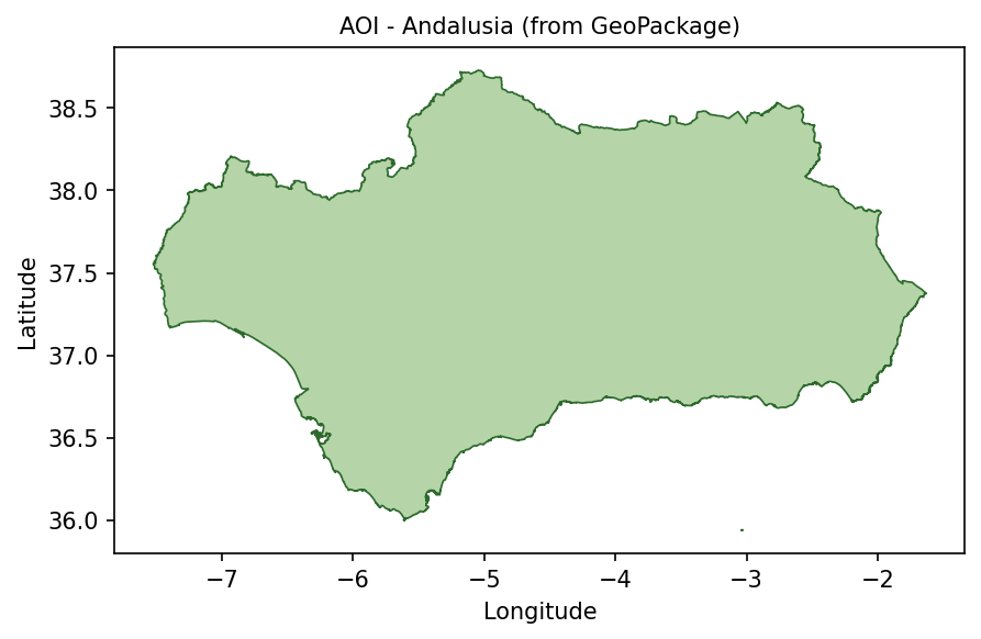
Andalusia area of interest loaded from andalusia.gpkg.

The same polygon is later rasterized into a mask, so that pixels outside Andalusia do not influence the spectral index statistics.

Step 4. Search the STAC catalogue

The notebook searches the STAC catalogue for MODIS MCD43A4 scenes covering Andalusia in 2022.

search = catalog.search(
    collections=["modis-terraaqua-mcd43a4"],
    datetime=f"{YEAR}-01-01/{YEAR}-12-31",
    bbox=[AOI_MINX, AOI_MINY, AOI_MAXX, AOI_MAXY],
    limit=5000,
    max_items=5000,
)

all_items = [
    item
    for item in search.items()
    if TILE_ID in item.id
]

all_items.sort(key=lambda item: item.properties["datetime"])

print(f"Items after tile filter: {len(all_items)}")

by_date = defaultdict(list)

for item in all_items:
    by_date[item.properties["datetime"][:10]].append(item)

all_dates = sorted(by_date.keys())

selected_dates = [
    all_dates[i]
    for i in np.linspace(0, len(all_dates) - 1, SCENES_TOTAL).astype(int)
]

selected_items = [
    by_date[date][0]
    for date in selected_dates
]

print(f"Selected dates: {len(selected_dates)}")
print(f"First date    : {selected_dates[0]}")
print(f"Last date     : {selected_dates[-1]}")

The selection distributes scenes across the year, giving an approximate intra-annual profile without downloading every available daily product.

Step 5. Download HDF4 files from S3

Each selected scene is downloaded from S3 into the local cache directory. Files that already exist are skipped.

def download_item(item):
    href = item.assets["data"].href
    path = href.removeprefix("s3:/").lstrip("/")
    bucket, key = path.split("/", 1)

    local_path = CACHE_DIR / os.path.basename(key)

    if not local_path.exists():
        s3.download_file(bucket, key, str(local_path))

    return item.id, local_path

local_paths = {}
total = len(selected_items)
done = 0
t_start = datetime.now()

with ThreadPoolExecutor(max_workers=4) as executor:
    futures = {
        executor.submit(download_item, item): item
        for item in selected_items
    }

    for future in as_completed(futures):
        item_id, local_path = future.result()
        local_paths[item_id] = local_path

        done += 1
        pct = done / total if total else 0
        bar = "█" * int(pct * 30) + "░" * (30 - int(pct * 30))

        clear_output(wait=True)
        print(f"[{bar}] {done}/{total} ({pct * 100:.1f}%)")

print(f"Downloaded or reused {len(local_paths)} files")

This step may take time on the first run. Later runs are faster because cached files are reused.

Step 6. Read HDF4 files and compute spectral indices

For each downloaded scene, the notebook:

1. opens the HDF4 file,

2. reads selected MODIS reflectance bands,

3. applies scale and fill-value handling,

4. clips the data to the area of interest,

5. applies the Andalusia polygon mask,

6. computes NDVI, EVI, and NDWI,

7. stores mean and standard deviation values for plotting.

Define the band and index helpers:

LAYER_TMPL = "Nadir_Reflectance_Band{}"
SCALE = 0.0001
FILL = 32767

def read_band(hdf, band_num, row0, row1, col0, col1):
    """Read one spectral band, clip it, and apply scaling."""
    sds = hdf.select(LAYER_TMPL.format(band_num))
    arr = sds[row0:row1, col0:col1].astype(np.float32)
    sds.endaccess()

    return np.where(arr == FILL, np.nan, arr * SCALE)

def safe_ratio(num, den):
    """Return num / den while avoiding invalid divisions."""
    with np.errstate(invalid="ignore", divide="ignore"):
        return np.where(np.abs(den) > 1e-9, num / den, np.nan)

Define a processing function for one selected item:

def process_item(item):
    hdf = None

    try:
        local_path = local_paths[item.id]
        hdf = SD(str(local_path), SDC.READ)

        h = w = 2400
        img_minx, img_miny, img_maxx, img_maxy = item.bbox

        col0 = max(0, min(w, int((AOI_MINX - img_minx) / (img_maxx - img_minx) * w)))
        col1 = max(0, min(w, int((AOI_MAXX - img_minx) / (img_maxx - img_minx) * w)))
        row0 = max(0, min(h, int((img_maxy - AOI_MAXY) / (img_maxy - img_miny) * h)))
        row1 = max(0, min(h, int((img_maxy - AOI_MINY) / (img_maxy - img_miny) * h)))

        if col1 <= col0 or row1 <= row0:
            return None

        red = read_band(hdf, 1, row0, row1, col0, col1)
        nir = read_band(hdf, 2, row0, row1, col0, col1)
        blue = read_band(hdf, 3, row0, row1, col0, col1)
        green = read_band(hdf, 4, row0, row1, col0, col1)
        swir = read_band(hdf, 6, row0, row1, col0, col1)

        transform = from_bounds(
            AOI_MINX,
            AOI_MINY,
            AOI_MAXX,
            AOI_MAXY,
            red.shape[1],
            red.shape[0],
        )

        mask = geometry_mask(
            [aoi_geojson],
            transform=transform,
            invert=False,
            out_shape=red.shape,
        )

        for arr in [red, nir, blue, green, swir]:
            arr[mask] = np.nan

        ndvi = safe_ratio(nir - red, nir + red)
        evi = 2.5 * safe_ratio(nir - red, nir + 6 * red - 7.5 * blue + 1)
        ndwi = safe_ratio(nir - swir, nir + swir)

        dt = datetime.fromisoformat(
            item.properties["datetime"].replace("Z", "+00:00")
        )

        return {
            "dt": dt,
            "month": dt.month,
            "red_arr": red,
            "green_arr": green,
            "blue_arr": blue,
            "ndvi_arr": ndvi,
            "evi_arr": evi,
            "ndwi_arr": ndwi,
            "ndvi_mean": float(np.nanmean(ndvi)),
            "evi_mean": float(np.nanmean(evi)),
            "ndwi_mean": float(np.nanmean(ndwi)),
            "ndvi_std": float(np.nanstd(ndvi)),
            "evi_std": float(np.nanstd(evi)),
            "ndwi_std": float(np.nanstd(ndwi)),
        }

    except Exception:
        return None

    finally:
        try:
            if hdf:
                hdf.end()
        except Exception:
            pass

Process all selected scenes:

results = []
total = len(selected_items)

with ThreadPoolExecutor(max_workers=4) as executor:
    futures = {
        executor.submit(process_item, item): item
        for item in selected_items
    }

    for i, future in enumerate(as_completed(futures), start=1):
        result = future.result()

        if result is not None:
            results.append(result)

        pct = i / total if total else 0
        bar = "█" * int(pct * 30) + "░" * (30 - int(pct * 30))

        clear_output(wait=True)
        print(f"[{bar}] {i}/{total} ({pct * 100:.1f}%)")

        if i % 20 == 0:
            gc.collect()

results = sorted(results, key=lambda r: r["dt"])

print(f"Processed scenes: {len(results)}")

The results list now contains spectral index arrays and statistics for each selected MODIS scene.

Step 7. Create a three-panel animated GIF

The animation combines three views for each date:

• true-colour RGB,

• NDVI,

• NDWI.

This makes it easier to compare the visual appearance of the landscape with vegetation and moisture signals.

def stretch(band):
    valid = band[~np.isnan(band)]

    if valid.size == 0:
        return np.full_like(band, 0.5)

    lo, hi = np.percentile(valid, [2, 98])

    return np.where(
        np.isnan(band),
        0.5,
        np.clip((band - lo) / (hi - lo + 1e-9), 0, 1),
    )

def make_triptych_frame(record):
    rgb = np.dstack(
        [
            stretch(record["red_arr"]),
            stretch(record["green_arr"]),
            stretch(record["blue_arr"]),
        ]
    )

    fig, axes = plt.subplots(1, 3, figsize=(18, 5))

    axes[0].imshow(rgb)
    axes[0].set_title("True colour")

    im1 = axes[1].imshow(record["ndvi_arr"], cmap="RdYlGn", vmin=-0.3, vmax=0.8)
    axes[1].set_title("NDVI")

    im2 = axes[2].imshow(record["ndwi_arr"], cmap="BrBG", vmin=-0.5, vmax=0.5)
    axes[2].set_title("NDWI")

    for ax in axes:
        ax.axis("off")

    fig.suptitle(record["dt"].strftime("%Y-%m-%d"))

    fig.canvas.draw()

    frame = np.frombuffer(fig.canvas.tostring_rgb(), dtype=np.uint8)
    frame = frame.reshape(fig.canvas.get_width_height()[::-1] + (3,))

    plt.close(fig)

    return Image.fromarray(frame)

frames = [make_triptych_frame(record) for record in results]

if frames:
    frames[0].save(
        "modis_reflectance_andalusia.gif",
        save_all=True,
        append_images=frames[1:],
        duration=400,
        loop=0,
    )

Animated comparison of true-colour RGB, NDVI, and NDWI for Andalusia.

The animated output is useful for visually checking how vegetation and moisture conditions change through the year.

Step 8. Plot spectral index anomalies

The next chart shows anomalies relative to the annual median. This makes seasonal stress easier to see than raw index values alone.

dates = [record["dt"] for record in results]

def anomaly(key):
    values = np.array([record[key] for record in results])
    return values - np.median(values)

index_data = {
    "NDVI anomaly": {
        "mean": anomaly("ndvi_mean"),
        "std": np.array([record["ndvi_std"] for record in results]),
        "color": "#2d8a2d",
        "ylim": (-0.25, 0.25),
    },
    "EVI anomaly": {
        "mean": anomaly("evi_mean"),
        "std": np.array([record["evi_std"] for record in results]),
        "color": "#7d2eab",
        "ylim": (-0.25, 0.25),
    },
    "NDWI anomaly": {
        "mean": anomaly("ndwi_mean"),
        "std": np.array([record["ndwi_std"] for record in results]),
        "color": "#1a6fa8",
        "ylim": (-0.35, 0.35),
    },
}

for title, cfg in index_data.items():
    values = cfg["mean"]

    if len(values) >= 7:
        smooth = savgol_filter(values, 7, 2)
    else:
        smooth = values

    fig, ax = plt.subplots(figsize=(13, 3))

    ax.plot(
        dates,
        values,
        marker="o",
        ms=3,
        lw=0.7,
        color=cfg["color"],
        alpha=0.35,
        label="scene anomaly",
    )

    ax.plot(
        dates,
        smooth,
        lw=2.2,
        color=cfg["color"],
        label="smoothed trend",
    )

    ax.axhline(0, color="#888", lw=0.8)
    ax.axvspan(
        datetime(2022, 6, 15),
        datetime(2022, 9, 15),
        color="red",
        alpha=0.08,
        label="dry season",
    )

    ax.set_title(title)
    ax.set_ylim(*cfg["ylim"])
    ax.grid(True, alpha=0.25)
    ax.legend(fontsize=8)

    fig.tight_layout()
    plt.show()

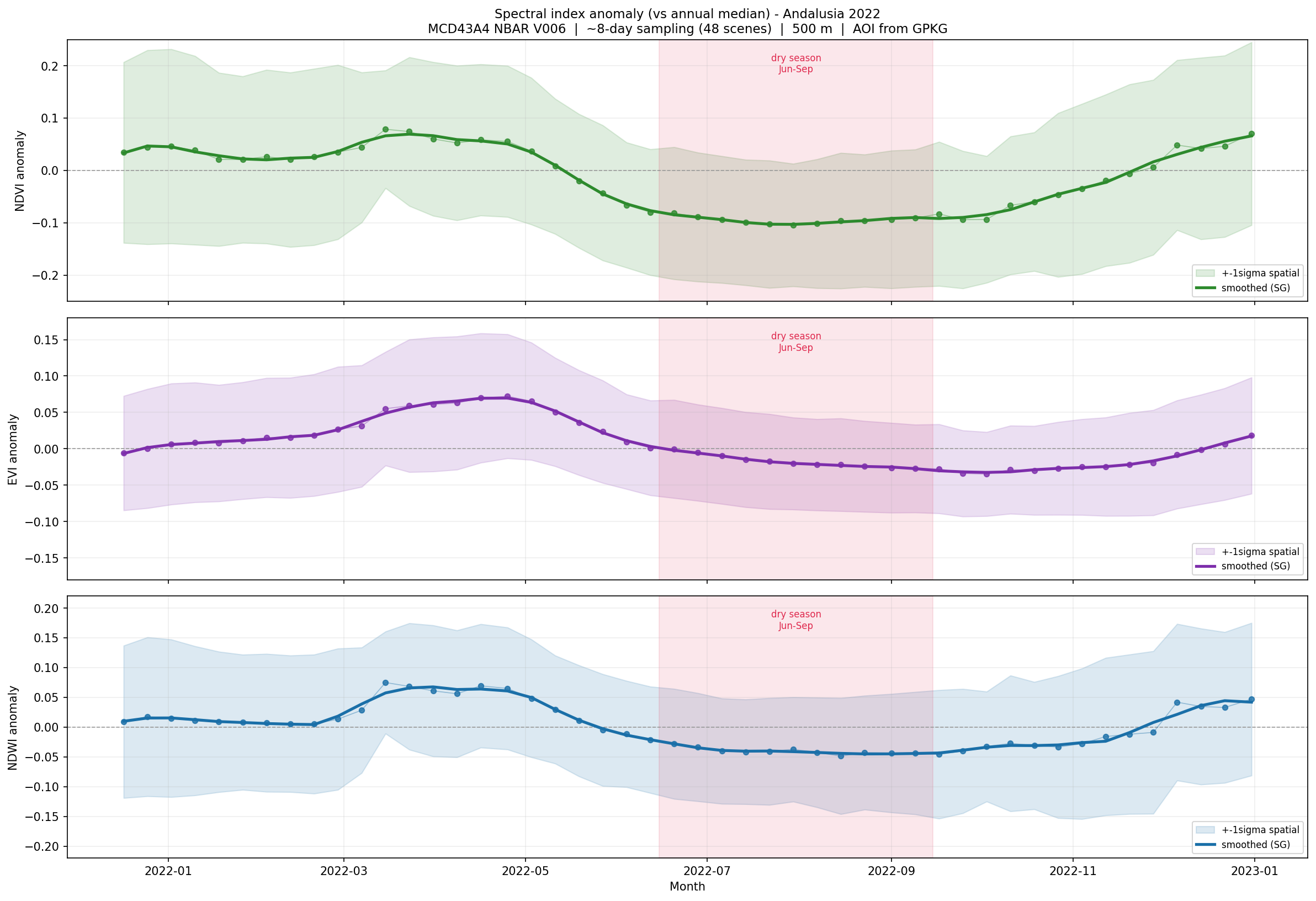
Spectral index anomalies for Andalusia during 2022, compared with the annual median.

Values above zero indicate greener or wetter-than-median conditions. Values below zero indicate lower greenness or stronger moisture stress.

Step 9. Plot monthly mean profiles

Monthly aggregation gives a compact overview of the seasonal cycle.

monthly = defaultdict(lambda: {"ndvi": [], "evi": [], "ndwi": []})

for record in results:
    monthly[record["month"]]["ndvi"].append(record["ndvi_mean"])
    monthly[record["month"]]["evi"].append(record["evi_mean"])
    monthly[record["month"]]["ndwi"].append(record["ndwi_mean"])

months = sorted(monthly.keys())
month_names = [datetime(2022, month, 1).strftime("%b") for month in months]
dry_months = {6, 7, 8, 9}

configs = [
    ("ndvi", "NDVI", "#2d8a2d"),
    ("evi", "EVI", "#7d2eab"),
    ("ndwi", "NDWI", "#1a6fa8"),
]

for key, label, color in configs:
    means = [
        np.mean(monthly[month][key])
        for month in months
    ]

    colors = [
        "#c0392b" if month in dry_months else color
        for month in months
    ]

    fig, ax = plt.subplots(figsize=(10, 3))

    bars = ax.bar(month_names, means, color=colors)

    for bar, value in zip(bars, means):
        ax.text(
            bar.get_x() + bar.get_width() / 2,
            value,
            f"{value:.2f}",
            ha="center",
            va="bottom",
            fontsize=8,
        )

    ax.set_title(f"Monthly mean {label} - Andalusia, 2022")
    ax.set_ylabel(label)
    ax.grid(True, alpha=0.25, axis="y")

    fig.tight_layout()
    plt.show()

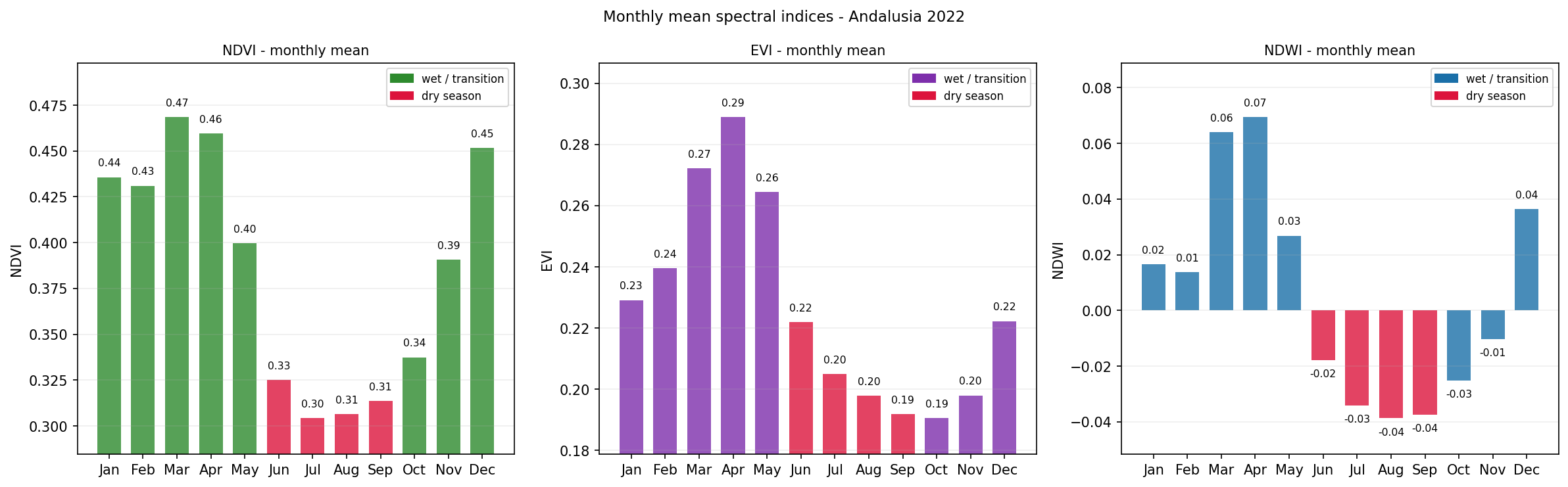
Monthly mean NDVI, EVI, and NDWI values for Andalusia in 2022.

The dry-season months are highlighted to make summer stress easier to identify.

Interpreting the results

The generated outputs provide several views of vegetation and moisture stress:

• The animated triptych compares true colour, NDVI, and NDWI for the same dates.

• The anomaly charts show when vegetation greenness and moisture depart from the annual median.

• The monthly profiles show how each index changes through the year.

• The dry-season highlighting helps connect the observed spectral response with seasonal drought pressure.

NDVI and EVI describe vegetation greenness. NDWI is more sensitive to vegetation water content. A sharp summer decline in NDWI, followed by lower NDVI and EVI, can indicate increasing moisture stress before visible greenness loss becomes obvious.

Limitations

Keep the following limitations in mind:

• MODIS reflectance data have a spatial resolution of 500 m.

• Spectral indices are indicators, not direct measurements of drought, desertification, or vegetation health.

• Atmospheric conditions, land-cover differences, irrigation, and topography can influence the index values.

• The workflow analyses one year only. Longer-term desertification analysis requires a multi-year time series.

• S3 credentials are required, and the notebook must be adapted if your S3 endpoint or credential method differs.

Conclusion

In this article, you used a Jupyter Notebook to analyze MODIS reflectance data over Andalusia. You searched the STAC catalogue, downloaded selected MODIS HDF4 files from S3, computed NDVI, EVI, and NDWI, and created outputs showing seasonal vegetation and moisture stress during 2022.

The same workflow can be reused for other regions, other years, and other MODIS reflectance-based studies.

What to do next

You can now adapt this workflow to your own analysis. For example, you can:

• replace andalusia.gpkg with another area-of-interest file,

• extend the analysis to multiple years,

• compare drought years with wetter baseline years,

• calculate additional indices such as NBR or SAVI,

• combine MODIS indices with ERA5 climate variables,

• export monthly index values for use in reports or dashboards.

You can also continue with other Python and Jupyter Notebook examples in the Cutting Edge section:

• Processing Sentinel-5P data on air pollution using Jupyter Notebook on Creodias

• Analyzing and monitoring floods using Python and Sentinel-2 satellite imagery on Creodias

• Monitoring Urban Sprawl with Sentinel-1 SAR Data Using Pixel Value and Polarization Thresholding on Creodias