MODIS active fire detection in Portugal using Jupyter Notebook on Creodias

Introduction

This article shows how to analyze MODIS active fire detections over mainland Portugal by using a Jupyter Notebook on Creodias. The example uses 8-day active fire composite products from MODIS Terra and Aqua for the period from 2003 to 2022.

The workflow searches the Copernicus Data Space STAC catalogue, identifies the MODIS products that cover Portugal, resolves their local paths on the virtual machine, and reads the HDF4 files directly from the mounted EODATA filesystem. This avoids a separate download step and makes the workflow suitable for multi-year fire analysis.

The area of interest is defined with the local GeoPackage file portugal.gpkg. The same polygon is used to derive the STAC search bounding box and to mask pixels outside the Portuguese border during processing.

Overview

The notebook processes two MODIS active fire products:

Product	Platform	Description
MOD14A2	Terra	8-day active fire composite
MYD14A2	Aqua	8-day active fire composite

Mainland Portugal spans two MODIS sinusoidal tiles:

Tile	Coverage
h17v04	Northern and central Portugal
h17v05	Southern Portugal

Both tiles are searched and processed. The Portugal polygon mask ensures that only pixels inside the Portuguese border contribute to the final statistics.

The analysis uses the MODIS FireMask layer and focuses on the following pixel classes:

Pixel value	Meaning
7	Low-confidence fire
8	Nominal-confidence fire
9	High-confidence fire
4	Cloud-obscured pixel
5	Non-fire land pixel

What you will do

In this article, you will:

• prepare a Python environment inside a Jupyter Notebook,

• load the Portugal area of interest from portugal.gpkg,

• search the STAC catalogue for MODIS Terra and Aqua active fire products,

• filter the result to the MODIS tiles that cover Portugal,

• resolve local HDF4 paths on the Creodias virtual machine,

• read and process the FireMask layer directly from /eodata,

• merge results from two MODIS tiles into national fire statistics,

• create time-series, annual, heatmap, and seasonality charts.

Prerequisites

Before starting, make sure that the following requirements are met.

No. 1 Hosting

You need a Creodias hosting account with access to the Horizon interface:

https://horizon.cloudferro.com/auth/login/?next=/

No. 2 Installing Jupyter Notebook

The code in this article runs in Jupyter Notebook. You can install it on your platform of choice by following the official Jupyter Notebook installation page.

One possible way to run Jupyter Notebook is to install it on a Kubernetes cluster. This is not required for completing this article, but the following article may be useful if you choose that setup:

Installing JupyterHub on Magnum Kubernetes Cluster in Creodias

No. 3 Access to EODATA

The notebook reads MODIS products from EODATA. Make sure that EODATA is available in the environment where you run Jupyter Notebook.

For this article specifically, the notebook reads local file paths from /eodata. Because of that, the first two articles below are the most important: they explain how to mount EODATA as a filesystem on a Linux virtual machine.

The credentials article is useful when the virtual machine does not already have EODATA configured. The catalogue-related article supports the discovery part of the workflow, where the catalogue is queried before the matching HDF4 files are processed locally.

Depending on how your environment is configured, you may need one of the following articles:

• How to mount EODATA as a filesystem using Goofys in Linux on Creodias

• How to mount eodata using s3fs in Linux on Creodias

• How to get credentials used for accessing EODATA on a cloud VM on Creodias

• EOData Catalogue API Manual on Creodias

No. 4 Notebook and support files

This article is accompanied by a ready-to-run Jupyter Notebook and the GeoPackage file used to define the area of interest.

Download both files before running the workflow:

• Download the notebook

• Download the Portugal GeoPackage file

Keep both files in the same working directory. The notebook reads portugal.gpkg directly when it loads the Portugal area of interest.

Required files

The notebook and the GeoPackage file must be available in the same working directory before you start running the code cells.

The GeoPackage file defines the Portugal area of interest. The notebook uses it twice: first to limit the STAC catalogue search to the selected area, and later to mask MODIS pixels outside Portugal during processing.

Step 1. Install dependencies

The notebook uses Python packages for STAC catalogue search, geospatial processing, HDF4 reading, plotting, and numerical analysis.

Run the following cell at the beginning of the notebook:

import importlib, subprocess, sys

pkgs = [
    "pystac_client",
    "pyhdf",
    "matplotlib",
    "numpy",
    "scipy",
    "geopandas",
    "shapely",
    "rasterio",
]

missing = [p for p in pkgs if importlib.util.find_spec(p) is None]

if missing:
    subprocess.check_call([sys.executable, "-m", "pip", "install", "-q"] + missing)

The packages are used as follows:

Package	Purpose
pystac_client	Queries the STAC catalogue and discovers matching MODIS scenes.
pyhdf	Reads HDF4 files produced by MODIS.
geopandas and shapely	Load the Portugal polygon and prepare the area of interest.
rasterio	Rasterizes the area-of-interest polygon into a pixel mask.
matplotlib	Creates the charts in the notebook.
numpy and scipy	Support numerical processing and time-series analysis.

Step 2. Import libraries and define global settings

After installing the packages, import the required libraries and define the global settings used by the workflow.

import gc
import os
import time
import numpy as np
import matplotlib.pyplot as plt
import matplotlib.patches as mpatches
import pystac_client
import geopandas as gpd

from shapely.geometry import mapping
from pyhdf.SD import SD, SDC
from datetime import datetime
from collections import defaultdict
from concurrent.futures import ThreadPoolExecutor, as_completed
from IPython.display import clear_output
from rasterio.transform import from_bounds
from rasterio.features import geometry_mask
from pathlib import Path

URL = "https://stac.dataspace.copernicus.eu/v1/"

catalog = pystac_client.Client.open(URL)
catalog.add_conforms_to("ITEM_SEARCH")

TILE_IDS = ["h17v04", "h17v05"]
MAX_WORKERS = min(8, os.cpu_count() or 4)
GC_EVERY = 50
LAYER = "FireMask"

FIRE_EVENTS = [
    (datetime(2003, 8, 1), "2003 season"),
    (datetime(2005, 8, 1), "2005 season"),
    (datetime(2017, 6, 17), "Pedrógão 2017-Jun"),
    (datetime(2017, 10, 15), "2017-Oct megafire"),
    (datetime(2022, 7, 12), "2022 season"),
]

print("ready")
print(f"Tiles   : {TILE_IDS}")
print(f"Workers : {MAX_WORKERS}")
print(f"Layer   : {LAYER}")

The most important setting is LAYER. It tells the notebook to read the FireMask scientific dataset from each MODIS HDF4 file.

Step 3. Load the Portugal area of interest

The area of interest is stored in portugal.gpkg. The notebook loads the file, reprojects it to WGS84 if needed, dissolves all features into one geometry, and extracts the bounding box used for the STAC search.

BASE_DIR = Path.cwd()
GPKG_PATH = BASE_DIR / "portugal.gpkg"

if not GPKG_PATH.exists():
    print(f"Warning: {GPKG_PATH} not found!")

aoi_gdf = gpd.read_file(GPKG_PATH)

if aoi_gdf.crs is None or aoi_gdf.crs.to_epsg() != 4326:
    aoi_gdf = aoi_gdf.to_crs(epsg=4326)

aoi_union = aoi_gdf.geometry.unary_union
aoi_geojson = mapping(aoi_union)

AOI_MINX, AOI_MINY, AOI_MAXX, AOI_MAXY = aoi_union.bounds

print(f"Loaded  : {GPKG_PATH}")
print(f"CRS     : {aoi_gdf.crs}")
print(f"Features: {len(aoi_gdf)}")
print(
    f"BBox    : lon [{AOI_MINX:.3f}, {AOI_MAXX:.3f}] "
    f"lat [{AOI_MINY:.3f}, {AOI_MAXY:.3f}]"
)

Display the polygon to verify that the correct area has been loaded:

fig, ax = plt.subplots(figsize=(5, 7))

aoi_gdf.plot(
    ax=ax,
    facecolor="#d4e8a0",
    edgecolor="#2d6a00",
    linewidth=0.8,
)

ax.set_title("AOI - Portugal from GeoPackage", fontsize=10)
ax.set_xlabel("Longitude")
ax.set_ylabel("Latitude")

plt.tight_layout()
plt.show()

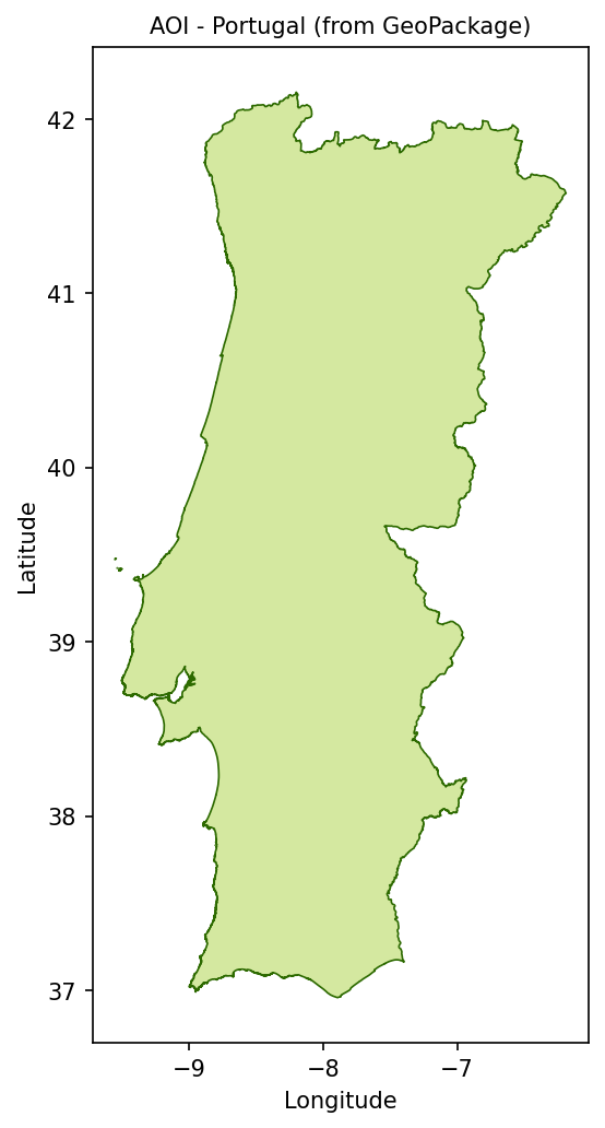
Portugal area of interest loaded from portugal.gpkg.

This polygon is important because the MODIS tiles extend beyond Portugal. The mask removes pixels over Spain, the Atlantic Ocean, and other areas outside the Portuguese border.

Step 4. Search the STAC catalogue

The notebook searches the Copernicus Data Space STAC catalogue for Terra and Aqua active fire products.

search = catalog.search(
    collections=["modis-terra-mod14a2", "modis-aqua-myd14a2"],
    datetime="2003-01-01/2022-12-31",
    bbox=[AOI_MINX, AOI_MINY, AOI_MAXX, AOI_MAXY],
    limit=6000,
    max_items=6000,
)

all_items = list(search.items())

items = [
    item
    for item in all_items
    if any(tile_id in item.id for tile_id in TILE_IDS)
]

items.sort(key=lambda item: item.properties["datetime"])

print(f"Items returned by STAC : {len(all_items)}")
print(f"Items after tile filter: {len(items)}")

if items:
    print(
        f"Date range: "
        f"{items[0].properties['datetime'][:10]} -> "
        f"{items[-1].properties['datetime'][:10]}"
    )

    platforms = set(item.properties.get("platform", "?") for item in items)
    tiles_found = set(
        tile_id
        for tile_id in TILE_IDS
        for item in items
        if tile_id in item.id
    )

    print(f"Platforms  : {platforms}")
    print(f"Tiles found: {tiles_found}")

The STAC query returns MODIS products that intersect the Portugal bounding box. The additional tile filter keeps only the two MODIS tiles needed for mainland Portugal.

Step 5. Read and process the HDF4 files

The MODIS files are read directly from EODATA. There is no separate download step.

For each composite, the notebook:

1. resolves the local filesystem path from the STAC asset link,

2. opens the HDF4 file with pyhdf,

3. converts the Portugal bounding box to row and column indices,

4. reads only the relevant window from the MODIS tile,

5. applies the Portugal polygon mask,

6. counts pixels in the selected FireMask classes.

First, define a helper function that converts the area of interest into a pixel window within each MODIS tile:

def window_for_item(item):
    """Return row and column indices that clip a MODIS tile to the AOI."""
    h = w = 1200
    img_minx, img_miny, img_maxx, img_maxy = item.bbox

    col0 = max(0, min(w, int((AOI_MINX - img_minx) / (img_maxx - img_minx) * w)))
    col1 = max(0, min(w, int((AOI_MAXX - img_minx) / (img_maxx - img_minx) * w)))
    row0 = max(0, min(h, int((img_maxy - AOI_MAXY) / (img_maxy - img_miny) * h)))
    row1 = max(0, min(h, int((img_maxy - AOI_MINY) / (img_maxy - img_miny) * h)))

    return row0, row1, col0, col1

Build the polygon masks once for each MODIS tile:

tile_masks = {}

for tile_id in TILE_IDS:
    representative_item = next((item for item in items if tile_id in item.id), None)

    if representative_item is None:
        continue

    row0, row1, col0, col1 = window_for_item(representative_item)

    if row1 > row0 and col1 > col0:
        nrows, ncols = row1 - row0, col1 - col0

        transform = from_bounds(
            AOI_MINX,
            AOI_MINY,
            AOI_MAXX,
            AOI_MAXY,
            ncols,
            nrows,
        )

        tile_masks[tile_id] = geometry_mask(
            [aoi_geojson],
            transform=transform,
            invert=False,
            out_shape=(nrows, ncols),
        )

        print(
            f"AOI mask for {tile_id}: {nrows}x{ncols} px "
            f"({tile_masks[tile_id].sum()} px outside AOI)"
        )

Then define the processing function for one STAC item:

def process_item(item):
    """Read one HDF file, clip it to the AOI, and count fire pixels."""
    hdf = sds = None

    try:
        local_path = item.assets["data"].href.removeprefix("s3:/")

        hdf = SD(str(local_path), SDC.READ)
        sds = hdf.select(LAYER)

        row0, row1, col0, col1 = window_for_item(item)

        if col1 <= col0 or row1 <= row0:
            return None

        arr = sds[row0:row1, col0:col1].copy()

        tile = next((tile_id for tile_id in TILE_IDS if tile_id in item.id), None)

        if tile and tile in tile_masks and arr.shape == tile_masks[tile].shape:
            arr[tile_masks[tile]] = 0

        dt = datetime.fromisoformat(
            item.properties["datetime"].replace("Z", "+00:00")
        )

        platform = item.properties.get("platform", "").lower()

        return {
            "dt": dt,
            "year": dt.year,
            "month": dt.month,
            "doy": dt.timetuple().tm_yday,
            "platform": "terra" if "terra" in platform else "aqua",
            "tile": tile,
            "fire_low": int(np.sum(arr == 7)),
            "fire_nom": int(np.sum(arr == 8)),
            "fire_high": int(np.sum(arr == 9)),
            "fire_total": int(np.sum((arr == 7) | (arr == 8) | (arr == 9))),
            "cloud_px": int(np.sum(arr == 4)),
            "land_px": int(np.sum(arr == 5)),
        }

    except Exception:
        return None

    finally:
        try:
            if sds:
                sds.endaccess()
        except Exception:
            pass

        try:
            if hdf:
                hdf.end()
        except Exception:
            pass

Process all items in parallel:

results = []
processed = 0
total = len(items)
t_start = datetime.now()
last_print_t = time.time()

PRINT_EVERY = 25
PRINT_EVERY_S = 5

with ThreadPoolExecutor(max_workers=MAX_WORKERS) as executor:
    futures = {executor.submit(process_item, item): item for item in items}

    for future in as_completed(futures):
        processed += 1
        result = future.result()

        if result is not None:
            results.append(result)

        now = time.time()

        if (
            processed % PRINT_EVERY == 0
            or (now - last_print_t) >= PRINT_EVERY_S
            or processed == total
        ):
            skipped = processed - len(results)
            elapsed = (datetime.now() - t_start).total_seconds()
            rate = processed / elapsed if elapsed > 0 else 0
            eta = (total - processed) / rate if rate > 0 else 0
            pct = processed / total if total else 0

            bar = "█" * int(pct * 30) + "░" * (30 - int(pct * 30))

            clear_output(wait=True)

            print(
                f"[{bar}] {processed}/{total} ({pct * 100:.1f}%)\n"
                f"  ok={len(results)}  skip={skipped}\n"
                f"  elapsed={elapsed:.1f}s  rate={rate:.1f} file/s  ETA={eta:.0f}s"
            )

            last_print_t = now

        if processed % GC_EVERY == 0:
            gc.collect()

gc.collect()

results = sorted(results, key=lambda r: r["dt"])

print(f"Done - {len(results)} results, {len(items) - len(results)} skipped")

The results list contains one record per valid MODIS file and tile.

Step 6. Build aggregate time series

Portugal spans two MODIS tiles. Before plotting, the notebook merges the two tiles per date and platform. This produces one national fire count for each 8-day composite.

merged = defaultdict(
    lambda: {
        "dt": None,
        "year": None,
        "month": None,
        "doy": None,
        "platform": None,
        "fire_low": 0,
        "fire_nom": 0,
        "fire_high": 0,
        "fire_total": 0,
        "cloud_px": 0,
        "land_px": 0,
    }
)

for r in results:
    key = (r["dt"].date(), r["platform"])
    m = merged[key]

    m["dt"] = r["dt"]
    m["year"] = r["year"]
    m["month"] = r["month"]
    m["doy"] = r["doy"]
    m["platform"] = r["platform"]

    m["fire_low"] += r["fire_low"]
    m["fire_nom"] += r["fire_nom"]
    m["fire_high"] += r["fire_high"]
    m["fire_total"] += r["fire_total"]
    m["cloud_px"] += r["cloud_px"]
    m["land_px"] += r["land_px"]

merged_results = sorted(merged.values(), key=lambda r: r["dt"])

yearly = defaultdict(lambda: {"low": 0, "nom": 0, "high": 0})
monthly = defaultdict(lambda: defaultdict(int))
ydoy = defaultdict(lambda: defaultdict(list))

for r in merged_results:
    y, m = r["year"], r["month"]

    yearly[y]["low"] += r["fire_low"]
    yearly[y]["nom"] += r["fire_nom"]
    yearly[y]["high"] += r["fire_high"]

    monthly[y][m] += r["fire_total"]
    ydoy[y][r["doy"]].append(r["fire_total"])

years = sorted(yearly.keys())

print(f"Years in analysis : {years[0]}-{years[-1]}")
print(f"Merged composites : {len(merged_results)}")
print(
    f"Peak fire year    : "
    f"{max(years, key=lambda y: yearly[y]['high'])} "
    f"(by high-confidence pixels)"
)

The aggregated datasets support several views of the fire record: Terra versus Aqua comparison, annual activity by confidence class, monthly heatmap, and seasonality by year.

Step 7. Plot Terra and Aqua fire detections

The first chart compares Terra and Aqua fire detections through time.

dates_t = [r["dt"] for r in merged_results if r["platform"] == "terra"]
fire_t = [r["fire_total"] for r in merged_results if r["platform"] == "terra"]

dates_a = [r["dt"] for r in merged_results if r["platform"] == "aqua"]
fire_a = [r["fire_total"] for r in merged_results if r["platform"] == "aqua"]

fig, ax = plt.subplots(figsize=(16, 5))

ax.plot(
    dates_t,
    fire_t,
    marker="o",
    ms=2.5,
    lw=0.7,
    label="Terra (MOD14A2)",
    color="#c0392b",
    alpha=0.8,
)

ax.plot(
    dates_a,
    fire_a,
    marker="x",
    ms=2.5,
    lw=0.7,
    label="Aqua (MYD14A2)",
    color="#e67e22",
    alpha=0.8,
)

ymax = ax.get_ylim()[1] or 1

for dt, label in FIRE_EVENTS:
    ax.axvline(dt, color="#555", lw=1, ls="--", alpha=0.5)
    ax.text(
        dt,
        ymax * 0.88,
        f" {label}",
        fontsize=7.5,
        color="#555",
        rotation=90,
        va="top",
    )

ax.set_xlabel("Date")
ax.set_ylabel("Fire pixels within AOI")
ax.set_title("Terra vs Aqua active fire detections - Portugal (2003-2022)")
ax.legend(fontsize=9)
ax.grid(True, alpha=0.25)

fig.tight_layout()
plt.show()

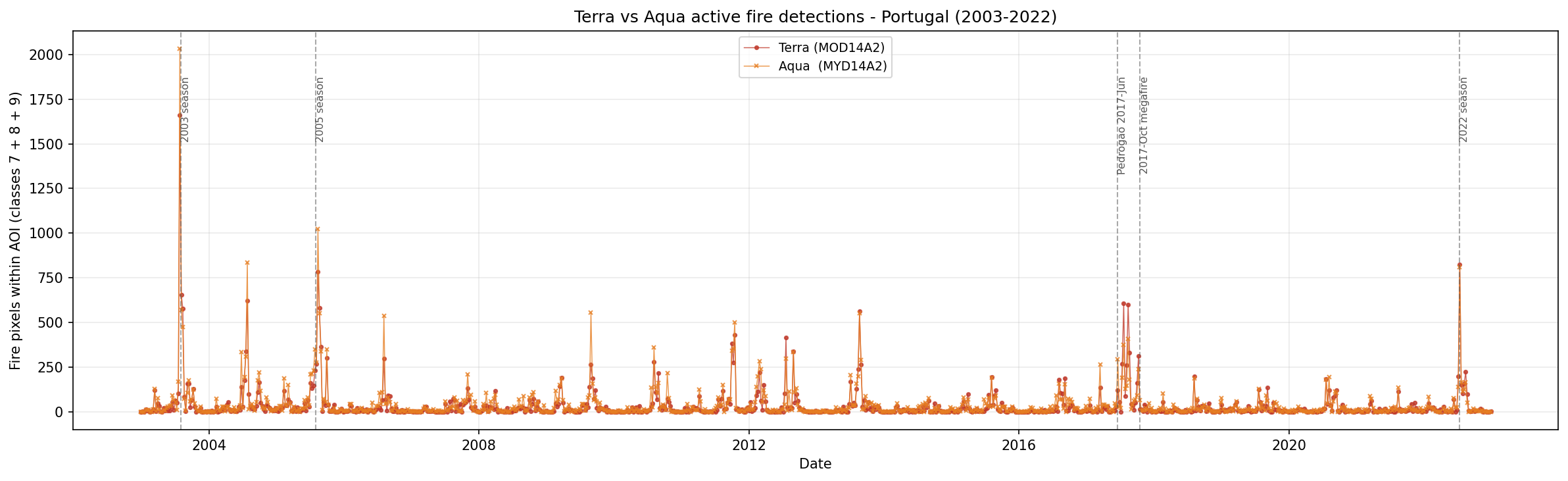
Terra and Aqua active fire detections over Portugal between 2003 and 2022.

Each point represents one 8-day composite. Major fire seasons should appear as clear spikes in the time series.

Step 8. Plot annual fire activity by confidence

The next chart shows annual fire-pixel counts split by confidence class.

years = [y for y in sorted(yearly.keys()) if 2003 <= y <= 2022]

x = np.arange(len(years))
bar_w = 0.28

fig, ax = plt.subplots(figsize=(16, 5))

ax.bar(
    x - bar_w,
    [yearly[y]["low"] for y in years],
    bar_w,
    label="Low confidence (7)",
    color="#f1c40f",
)

ax.bar(
    x,
    [yearly[y]["nom"] for y in years],
    bar_w,
    label="Nominal confidence (8)",
    color="#e67e22",
)

ax.bar(
    x + bar_w,
    [yearly[y]["high"] for y in years],
    bar_w,
    label="High confidence (9)",
    color="#c0392b",
)

ax.set_xticks(x)
ax.set_xticklabels(years, rotation=45, ha="right")
ax.set_xlabel("Year")
ax.set_ylabel("Fire pixel count within AOI")
ax.set_title("Annual fire activity by detection confidence - Portugal")
ax.legend(fontsize=9)
ax.grid(True, alpha=0.25, axis="y")

fig.tight_layout()
plt.show()

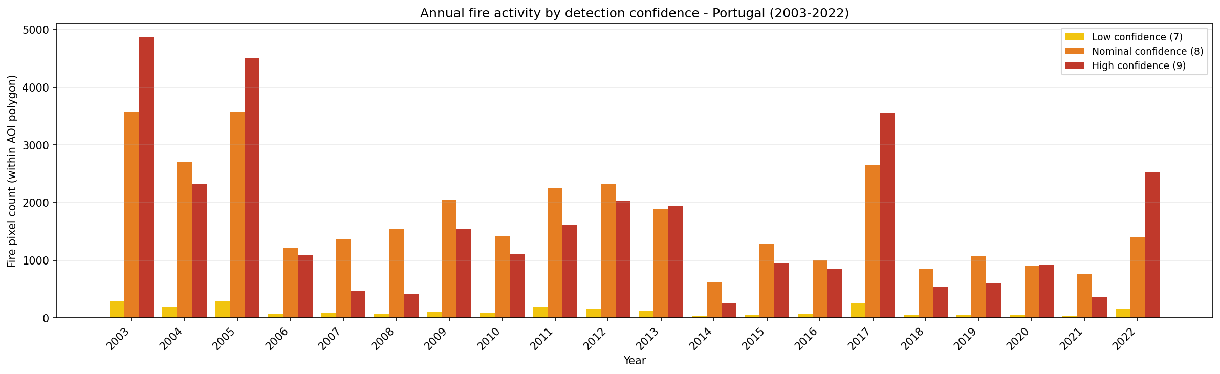
Annual fire activity in Portugal grouped by MODIS detection confidence class.

This chart separates possible, likely, and high-confidence fire detections. For summary analysis, the high-confidence class is often the most conservative indicator.

Step 9. Plot the year-month fire heatmap

The heatmap compresses 20 years of monthly fire activity into one view.

all_years = [y for y in sorted(monthly.keys()) if 2003 <= y <= 2022]

month_names = [
    "Jan", "Feb", "Mar", "Apr", "May", "Jun",
    "Jul", "Aug", "Sep", "Oct", "Nov", "Dec",
]

matrix = np.array(
    [
        [monthly[y].get(m, 0) for m in range(1, 13)]
        for y in all_years
    ],
    dtype=float,
)

fig, ax = plt.subplots(figsize=(13, 8))

im = ax.imshow(
    matrix,
    aspect="auto",
    cmap="YlOrRd",
    interpolation="nearest",
)

plt.colorbar(im, ax=ax, label="Total fire pixels within AOI")

ax.set_yticks(range(len(all_years)))
ax.set_yticklabels(all_years, fontsize=9)
ax.set_xticks(range(12))
ax.set_xticklabels(month_names)
ax.set_title("Fire activity heatmap - Portugal: year x month")

fig.tight_layout()
plt.show()

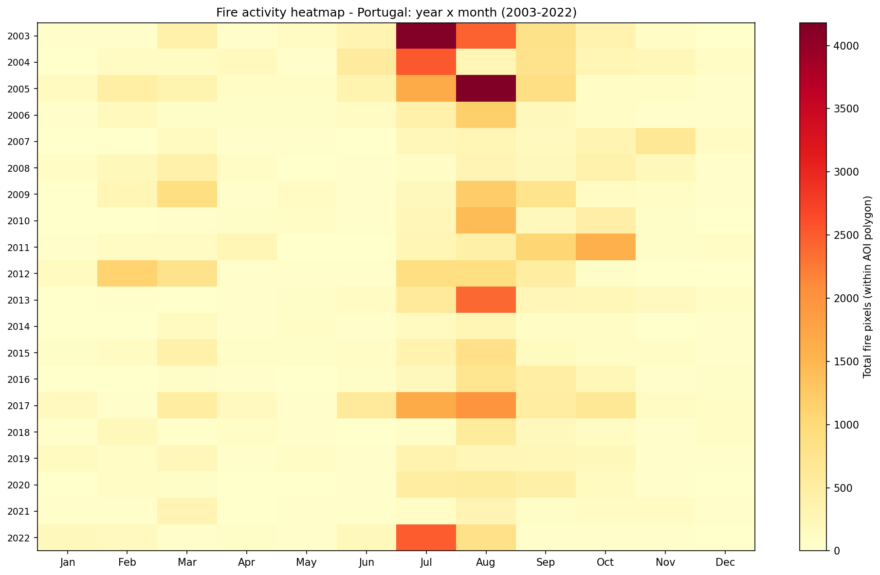
Monthly fire activity heatmap for Portugal from 2003 to 2022.

Bright cells indicate months with high fire activity. In Portugal, the strongest activity is expected during the summer fire season.

Step 10. Plot fire seasonality by year

The final chart shows the distribution of fire pixels through the calendar year.

all_plot_years = [y for y in sorted(ydoy.keys()) if 2003 <= y <= 2022]
fire_cmap = plt.colormaps["YlOrRd"].resampled(len(all_plot_years))

fig, ax = plt.subplots(figsize=(16, 5))

for j, y in enumerate(all_plot_years):
    doys = sorted(ydoy[y].keys())
    vals = [np.mean(ydoy[y][d]) for d in doys]

    ax.plot(
        doys,
        vals,
        lw=1.2,
        ms=3,
        marker="o",
        label=str(y),
        color=fire_cmap(j),
        alpha=0.85,
    )

ax.axvspan(152, 273, alpha=0.07, color="red")
ax.text(
    212,
    ax.get_ylim()[1] * 0.95,
    "Jun-Sep fire season",
    ha="center",
    fontsize=8,
    color="#c0392b",
    alpha=0.7,
)

ax.set_xlabel("Day of year")
ax.set_ylabel("Mean fire pixels per 8-day composite")
ax.set_title("Fire seasonality by year - Portugal")
ax.legend(ncol=4, fontsize=7.5, loc="upper left")
ax.grid(True, alpha=0.25)

fig.tight_layout()
plt.show()

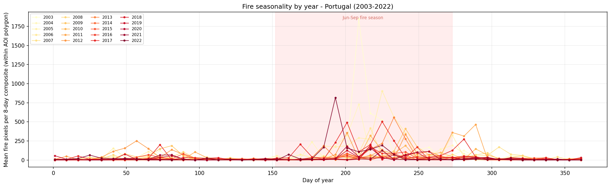
Seasonal distribution of MODIS fire detections in Portugal by year.

The shaded area marks the core fire season. Spikes outside this range may indicate early- or late-season events.

Interpreting the results

The generated charts provide several complementary views of fire activity in Portugal:

• The Terra versus Aqua chart shows the timing of active fire detections.

• The annual confidence chart compares fire activity between years.

• The heatmap shows which months contributed most to annual fire activity.

• The seasonality chart shows whether fire events occurred inside or outside the usual summer fire season.

The analysis counts classified MODIS fire pixels. It does not directly estimate burned area, fire severity, or damage, but it gives a useful satellite-based view of the timing and intensity of fire activity.

Limitations

Keep the following limitations in mind:

• MODIS active fire products detect thermal anomalies, not burned area.

• Cloud cover, smoke, and viewing geometry can affect detection.

• The 8-day composite interval is useful for long-term analysis, but it does not preserve all details of individual fire events.

• The workflow counts fire pixels inside the Portugal polygon. It does not replace official fire-perimeter or civil-protection datasets.

• The notebook reads files directly from /eodata, so it must be adapted if you want to run it outside the Creodias environment.

Conclusion

In this article, you used a Jupyter Notebook to analyze MODIS active fire detections over Portugal from 2003 to 2022. You searched the STAC catalogue, resolved the matching HDF4 files on the EODATA filesystem, processed the FireMask layer, and created charts showing annual, monthly, and seasonal patterns of fire activity.

The same structure can be adapted to other MODIS fire products, other regions, or other Earth observation datasets available on Creodias.

What to do next

You can now adapt this workflow to your own analysis. For example, you can:

• replace portugal.gpkg with another area-of-interest file,

• change the MODIS tile filters for another region,

• compare Terra and Aqua detections separately,

• focus only on high-confidence fire pixels,

• combine MODIS fire detections with drought, temperature, wind, or land-cover datasets,

• export the aggregated results for reporting or dashboard use.

You can also continue with other Python and Jupyter Notebook examples in the Cutting Edge section:

• Processing Sentinel-5P data on air pollution using Jupyter Notebook on Creodias

• Analyzing and monitoring floods using Python and Sentinel-2 satellite imagery on Creodias

• Monitoring Urban Sprawl with Sentinel-1 SAR Data Using Pixel Value and Polarization Thresholding on Creodias