Sample Deep Learning Workflow Using TensorFlow Running on Docker on Creodias vGPU Virtual Machine
This is a demonstration of using Deep Learning tools TensorFlow and Keras for performing custom image classification on vGPU in .
The use of (v)GPU will speed up the calculations involved in Deep Learning. In this example, it will cut down processing time from a couple of hours to a couple of minutes.
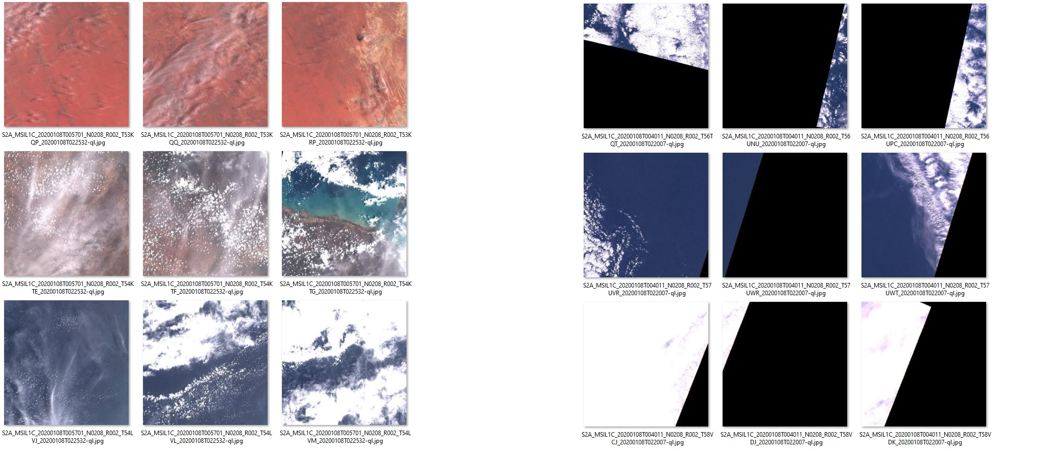
The task you are going to apply TensorFlow to is how to recognize which sets of images are cropped and which are not. In two sets of images shown below, the images on the left are not cropped while those on the right are cropped. The model you are going to develop in this article will be able to reach (more or less) the same conclusions as humans would for the same set of pictures.
Warning
Satellite image processing is a discipline of its own, utilizing various techniques. This article concentrates on absolute basics just to demonstrate the concept and a possible workflow when using Deep Learning on a vGPU machine.
Also, the model here developed is just an example. Using it in production would require extensive further testing. The model is not deterministic and will produce different results with each training.
If you want to perform this deep learning workflow without using Docker, visit the following articles instead: Install TensorFlow on vGPU enabled VM on Creodias and Sample Deep Learning workflow using vGPU and EO DATA on Creodias.
What We Are Going To Do
Provide thorough explanation of Python code used in this process
Use Docker as the environment for model development
Build a custom container image called deeplearning based on the public image tensorflow/tensorflow:2.11.0-gpu.
Download data for testing and training
Install our Python script deeplearning.py into the Docker container
Install the dependencies required by the app (pandas and numpy)
Run the model against the data you downloaded from this article
Analyze the results
Benchmark the model on flavors vm.a6000.1 and vm.a6000.8 and show that on the latter, the process is up to five times faster
Prerequisites
No. 1 Account
You need a Creodias hosting account with access to the Horizon interface: https://horizon.cloudferro.com/auth/login/?next=/.
No. 2 Create a New Linux VM With NVIDIA Virtual GPU
Here is how you can create a new Linux VM with vGPU: How To Create a New Linux VM With NVIDIA Virtual GPU in the OpenStack Dashboard Horizon on Creodias.
No. 3 Add a floating IP address to your VM
How to Add or Remove Floating IP’s to your VM on Creodias.
You will now be able to use that floating IP address for the examples in this article.
No. 4 TensorFlow installed on Docker
You need to have TensorFlow installed using Docker on a Creodias GPU-enabled virtual machine. The following article describes how it can be done: Install TensorFlow on Docker Running on Creodias vGPU Virtual Machine.
No. 5 Running locally on Ubuntu 20.04 LTS computer
This article assumes that your local computer is running Ubuntu 20.04 LTS. You can, however, run this model from any other operating system provided you use the relevant commands for file operations, SSH access and so on.
Code Explanation
This section contains detailed explanation of this process and the Python code used for it. For the practical steps allowing you to replicate this workflow, please start with the section Practical workflow (see below). You will not have to copy the Python code yourself, a file with it is available to download for your convenience.
Step 1: Data Preparation
Data Preparation is the fundamental (and usually most time-involved) step in each Data Science related project. In order for our DL model to be able to learn we will follow the typical (supervised learning) sequence:
Organize a sufficiently large sample of data (here: a Sentinel-2 satellite images sample).
Tag/Label this data manually (by human). In our example we manually separated the images to “edges” and “noedges” categories, representing cropped and non-cropped images respectively.
Put aside part of this data as Train(+Validation) subset, which will be used to “teach” the model.
Put aside another subset as Test. This is a control subset that model never sees during the learning phase, and will be used to evaluate model quality.
The downloadable .zip file found later in this article is an already prepared (according to these steps) dataset. It contains
592 files of Train/Validate set (50/50 cropped/non-cropped images)
148 files of Test set (also 50/50 cropped/non-cropped).
Based on the folder and sub-folder names from this dataset Keras will automatically entail the labels, so it is important to keep the folder structure as it is.
The final step is doing necessary operations on the data so that it is a proper input for the model. TensorFlow will do a lot of this work for us. For example, using the image_dataset_from_directory function, each image is automatically labeled and converted to a vector/matrix of numbers: height x width x depth (RGB layer).
For your specific use case you might need to do various optimizations of data along this step.
import numpy as np
import tensorflow as tf
from tensorflow import keras
import pandas as pd

# DATA INGESTION
# -------------------------------------------------------------------------------------
# Ingest the Training, Validation and Test datasets from image folders.
# The labels (edges vs. noedges) are automatically inferred based on folder names.

train_ds = keras.utils.image_dataset_from_directory(
  directory='./data/train',
  labels='inferred',
  label_mode='categorical',
  validation_split=0.2,
  subset='training',
  image_size=(343, 343),
  seed=123,
  batch_size=8)

val_ds = keras.utils.image_dataset_from_directory(
  directory='./data/train',
  labels='inferred',
  label_mode='categorical',
  validation_split=0.2,
  subset='validation',
  image_size=(343, 343),
  seed=123,
  batch_size=8)

test_ds = keras.utils.image_dataset_from_directory(
  directory='./data/test',
  labels='inferred',
  label_mode='categorical',
  image_size=(343, 343),
  shuffle = False,
  batch_size=1)
Step 2: Defining and Training of the Model
Defining an optimal model is the art and science of Data Science. What we are showing here is merely a simple sample model and you should read more from other sources about creating models for real life scenarios.
Once the model is defined, it gets compiled and its training begins. Each epoch is the next iteration of tuning the model. These epochs are complex and heavy computing operations. Using vGPU is fundamental for Deep Learning applications, as it enables distributing micro-tasks over hundreds of cores, thus speeding up the process immensely.
Once the model is fit we will save it and reuse for generating predictions.
# TRAINING
# -------------------------------------------------------------------------------------
# Build, compile and fit the Deep Learning model

model = keras.applications.Xception(
   weights=None, input_shape=(343, 343, 3), classes=2)
model.compile(optimizer='rmsprop', loss='categorical_crossentropy', metrics='accuracy')
model.fit(train_ds, epochs=5, validation_data=val_ds)

model.save('model_save.h5')

# to reuse the model later:
#model = keras.models.load_model('model_save.h5')
Step 3: Generating Predictions for the Test Data
Once the model has been trained, generating the predictions is a simple and much faster operation. As outlined before, we will use the model to generate predictions for the test data.
# GENERATE PREDICTIONS on previously unseen data
# -------------------------------------------------------------------------------------
predictions_raw = model.predict(test_ds)
Step 4: Summarizing the Results
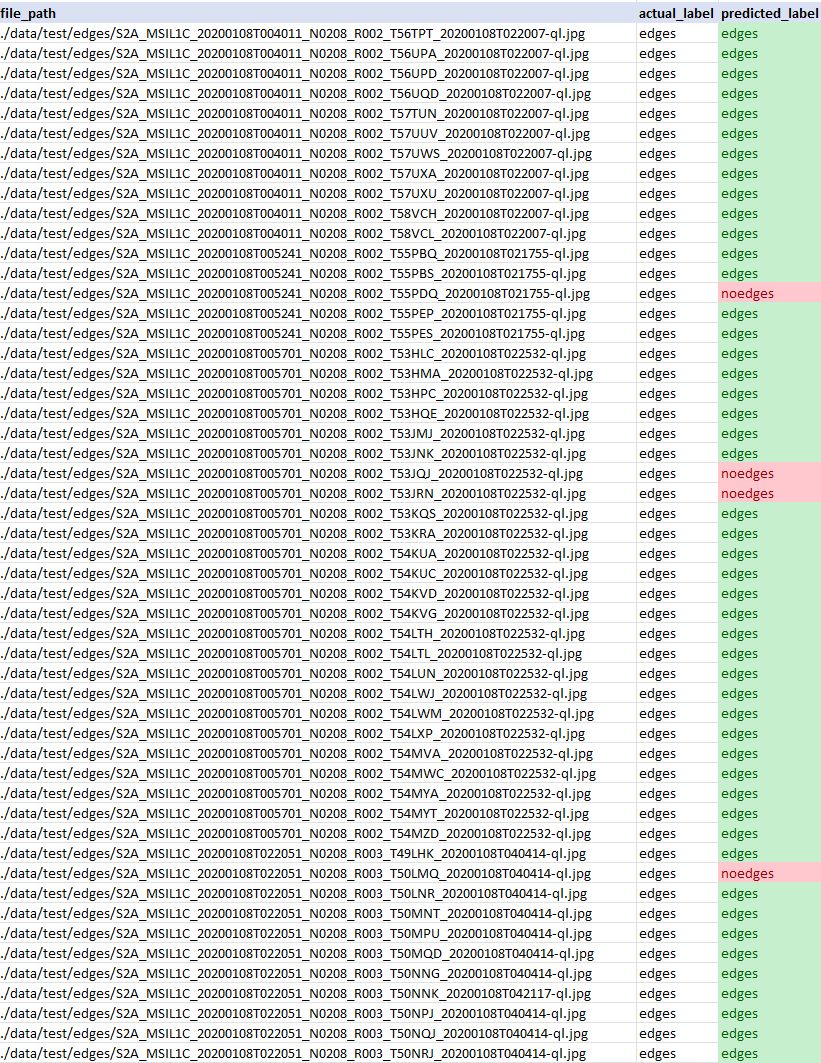
In this step we take the actual labels (“edges” vs. “noedges” which represent “cropped” vs. “non-cropped” images) and compare to the labels which our model predicted.
We summarize the results in a Data Frame saved as a CSV file, which enables interpreting actual results in the test set vs. the predictions provided by the model.
Example of CSV output:
# SUMMARIZE RESULTS (convenience, alternative approaches are available)
# -------------------------------------------------------------------------------------

# initialize pandas dataframe with file paths
df = pd.DataFrame(data = {"file_path": test_ds.file_paths})
class_names = test_ds.class_names # ["edges","noedges"]

# add actual labels column
def get_actual_label(label_vector):
    for index, value in enumerate(label_vector):
      if (value == 1):
          return class_names[index]
actual_label_vectors = np.concatenate([label for data, label in test_ds], axis=0).tolist() # returns array of label vectors [[0,1],[1,0],...] representing category (edges/noedges)
actual_labels =  list(map(lambda alv: get_actual_label(alv), actual_label_vectors))
df["actual_label"] = actual_labels


# add predicted labels column
predictions_binary = np.argmax(predictions_raw, axis=1) # flatten to 0-1 recommendation
predictions_labeled = list(map(lambda x: class_names[0] if x == 0 else class_names[1],list(predictions_binary)))

df["predicted_label"] = predictions_labeled


df.to_csv("results.csv", index=False)
Practical Workflow
This section contains practical steps which allow you to perform this workflow yourself. This is just an example and you can create a different workflow on your own.
Please revisit the Prerequisites section before undertaking the practical steps below.
You can transfer the required files to your virtual machine using different methods, such as:
- Download the files to your local computer and copy them using scp to your virtual machine
Click on the links below to download the data
- Download the files directly to your virtual machine using wget
This method will be described in Step 1.
Step 1: Download the resources to your virtual machine
Connect to your virtual machine using SSH (replace 64.225.129.70 with the floating IP address of your virtual machine).
ssh eouser@64.225.129.70
Note
Skip the rest of this step if you copied have already transferred the files to your virtual machine using a different method.
Download the required resources to your virtual machine using the following command:
wget https://creodias.docs.cloudferro.com/en/latest/_downloads/3ec8990b08af7d4478a6820abb172705/data.zip https://creodias.docs.cloudferro.com/en/latest/_downloads/1c3a17567b2f4f1ff87ddbbfe005db42/deeplearning.py
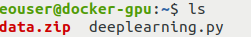
Execute the ls command to verify that the files you copied are there:
Step 2: Move the downloaded resources to the appropriate location
Create a folder called deeplearning on your VM in which you will place downloaded resources:
mkdir deeplearning
Use the following command to move the required files to that directory:
mv deeplearning.py data.zip deeplearning
Now, navigate to the folder you just created:
cd deeplearning
Step 3: Create a Dockerfile and file requirements.txt
Install the text editor nano if you haven’t already and create a Dockerfile using it in your current working directory (a text file called Dockerfile):
sudo apt install nano
nano Dockerfile
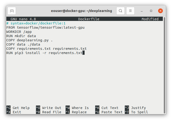
Paste the following code into it:
# syntax=docker/dockerfile:1
FROM tensorflow/tensorflow:2.11.0-gpu
WORKDIR /app
RUN mkdir data
COPY deeplearning.py .
COPY data ./data
COPY requirements.txt requirements.txt
RUN pip3 install -r requirements.txt
After pasting, your screen should look like this:
Save the file and exit nano using the following sequence of keys: press CTRL+X and press Y and then Enter.
Add text file requirements.txt to the same folder using the same method:
nano requirements.txt
Type the following content into the editor:
numpy==1.22.4
pandas==1.4.2
Using file requirements.txt is a standard way in Python to set up and install the extensions needed.
Save the file and exit nano in the same way as previously: CTRL+X, Y, Enter.
Step 4: Unzip and delete the archive containing the training data
Unzip the archive data.zip and then remove it:
unzip data.zip
rm data.zip
Step 5: Verify That All the Needed Files are in the Correct Place
Execute the ls command to verify that the following files are there:
folder data
file deeplearning.py.
file Dockerfile
file requirements.txt

Step 6: Build a Docker Image and Enter it
From the folder with the Dockerfile run the following command to build the container image:
sudo docker build -t deeplearning .
Then start the container with interactive shell:
sudo docker run -it --gpus all -v /tmp/:/tmp/ deeplearning /bin/bash
You should see the following output:
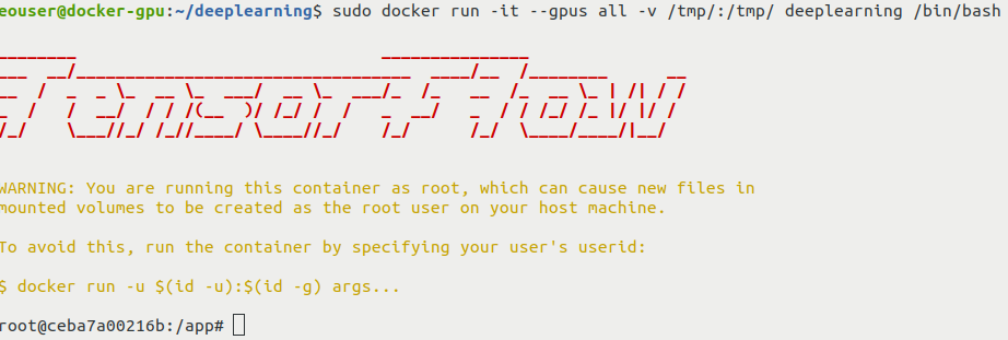
The option -v will mount a volume shared between your container and your host VM. This will enable copying of files generated by our script to the host VM.
Step 7: Run the Python code
From the inside of the container run the Python script:
python3 deeplearning.py
On a vGPU-enabled VM the execution of this script should last a couple of minutes. This operation should create a file results.csv containing the results. Additionally, to avoid repeating of training, the model is saved as a file named model_save.h5.
Step 8: Extract the Files From the Container
Once finished, the last step is to copy the files from the /tmp folder inside the container to the /tmp folder on the host machine. Execute the following command from the interactive container shell:
cp results.csv model_save.h5 /tmp
You can now leave the container using the following command:
exit
Now that you have left the container, go to the /tmp folder on your virtual machine:
cd /tmp
Use the ls command to verify that files results.csv and model_save.h5, containing the results of this operation, can be found there. We will copy them to your local computer in the next step.
You can now also disconnect from the virtual machine:
exit
Step 9: Download the File with the Results to Your Local Machine
You are now going to download the results and the saved model to your local machine. Make the folder that contains the file results.csv your current working directory, then execute the following command (replace 64.225.129.70 with the floating IP address of your virtual machine):
scp eouser@64.225.129.70:/tmp/results.csv eouser@64.225.129.70:/tmp/model_save.h5 .
The csv file containing the results and the file containing the model should now be on your local machine:
Performance Comparison
This article has the TensorFlow installed within a Docker environment. There is a parallel article with the same example running directly on WAW3-a cloud (Sample Deep Learning workflow using vGPU and EO DATA on Creodias) and we are now going to compare running times from these environments, using the smallest and the biggest flavors for vGPUs, vm.a6000.1 and vm.a6000.8.
The table below contains the amount of time it takes for the execution of Python code to be completed. It was measured using the time command (“real value”). All tests were performed on the Creodias cloud.
vm.a6000.1 |
vm.a6000.8 |
|
Docker used |
5m50.449s |
1m14.446s |
Docker not not used |
5m0.276s |
0m55.547s |
The whole process took then about 5 times less time on the vm.a6000.8 flavor than it took on the vm.a6000.1 flavor. There is a small penalty when using Docker, but that is expected.
Note
This benchmark counts all phases of the execution of the Python code and not all of them may benefit from better hardware to the same degree.
What Can Be Done Next
You can also perform this workflow without using Docker. If you want to do so, see the following article:
Sample Deep Learning workflow using vGPU and EO DATA on Creodias.
Warning
The samples in this article might be non-representative and your mileage may vary. Use this code and the entire article as a starting point to conduct your own research.