Using Sentinel-2 images to monitor mouth of the river Syr Darya and Aral Lake and analyzing it with NDWI index on Creodias
In this article, we will present a simple example on how you can easily access data from Creodias, using RESTO API. We will access Sentinel-2 images containing data of Syr Darya river and Aral Lake in Kazakhstan. Our goal will be to monitor daily quantity of water in the near area of that lake, from May to July 2023.
We will use Python packages to both obtain images from the cloud and analyze the water with the Normalized difference Water Index (NDWI).
What is NDWI?
NDWI is a normalized difference index calculated based on the reflectance of light in two different spectral bands: green (G) and near-infrared (NIR). The formula for calculating NDWI is as follows:
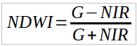
where:
G - reflectance in the green band,
NIR - reflectance in the near-infrared band.
NDWI values range from -1 to 1, where higher values indicate the presence of water, while the lower values may indicate other land cover types, such as vegetation or urban areas.
Advantages of using NDWI indicator
Raster images containing the NDWI indicator can be used in various fields, including:
- Water Resource Monitoring
Tracking changes in water levels in lakes, rivers, and reservoirs, especially important in areas affected by drought or excessive rainfall.
- Crisis Management
Rapid identification of flooded areas during floods and assessment of damages.
- Environmental Protection
Monitoring wetlands and other aquatic ecosystems to preserve their biodiversity.
- Urban Planning
Analyzing the impact of urban development on nearby water resources.
- Agriculture
Assessing irrigation of agricultural fields and monitoring plant health.
What We Are Going To Cover
Define variables to hold the data
Work with RESTO API
Create template for API URL
Create request from template
Obtain products’ paths
Obtain NDWI
Functions for reading, calculating and saving raster data
Computing NWDI rasters
Analysis
Prerequisites
No. 1 Hosting
You need a Creodias hosting account with access to the Horizon interface: https://horizon.cloudferro.com/auth/login/?next=/.
No. 2 A Jupyter Notebook operational
The code in this article runs on Jupyter Notebook and you can install it on your platform of choice by following the official Jupyter Notebook install page.
One particular way of installing (and by no means being required to follow up this article), is to install it on Kubernetes cluster. If that is the case, this article will be useful:
Installing JupyterHub on Magnum Kubernetes Cluster in Creodias .
You can download the entire code for this article and execute in your Jupyter Notebook, from this link:
No. 3 requests Python package operational
To connect with RESTO, we will use only one Python package – requests. It is a standard library that can send GET/POST requests to HTTP servers and handle responses.
If not already installed, install it withf
pip install requests
and then import it with the following command, somewhere in the beginning of the file:
import requests
No. 4 Installed python libraries for imagery data
Here are Python spatial-oriented packages we are going to use for imagery data:
- rasterio
Allows us to read raster data and to visualize created NDWI images.
- osgeo
A GDAL API for Python.
- numpy
Popular Python package, allowing complex math equations and formats, such as matrices.
- os
Connects Python to the Operating System.
Packages needed may be complicated to install (especially osgeo) so you may want to use conda environment. It is an open-source package and environment manager, shared by many geospatial packages.
Define variables to hold the data
We are interested in a period of time in which we are observing and analyzing the quantity of water in Syr Darya river and Aral Lake, as well as the corresponding area. The coordinates are defined through BBOX (Bounding Box), as a list of coordinates – Xmin, Ymin, Xmax, Ymax. All coordinates will be defined in EPSG:4326.
In python, we define three variables:
# Timerange of data that we want to recieve
start_date = '2023-05-01'
end_date = '2023-07-31'
# Geometry in form of a BBOX
bbox = [60.2347,46.1731,61.1160,46.6541]
This how it will, typically, look at the Jupyter Notebooks of choice:
Work with RESTO API
RESTO API is a way of communicating with EODATA, which is a vast repository of Earth Observation data. RESTO is an API built upon RESTful API and allows users to request data based on spatial and temporal parameters.
Create template for API URL
We will use this predefined template for requesting data. Some parameters are defined as variables, and we will be able to edit them.
API_URL = """http://datahub.creodias.eu/resto/api/collections/Sentinel2/search.json?\
box={minx},{miny},{maxx},{maxy}\
&startDate={start_date}\
&completionDate={end_date}\
&sortParam=startDate\
&sortOrder=ascending\
&platform=S2A\
&cloudCover=[0,10]"""
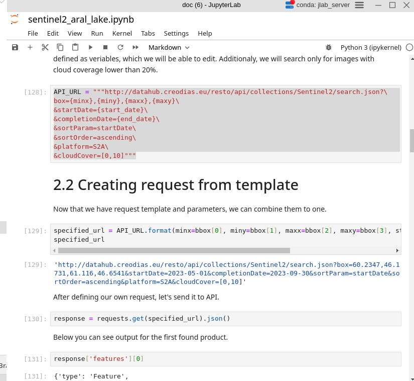
Creating request from template
Now that we have a request template and the values of its parameters, we can merge them into an actual command:
specified_url = API_URL.format(minx=bbox[0], miny=bbox[1], maxx=bbox[2], maxy=bbox[3], start_date=start_date, end_date=end_date)
The value of the obtained url is:
specified_url
`https://datahub.creodias.eu/resto/api/collections/Sentinel2/search.json?box=60.2347,46.1731,61.116,46.6541&startDate=2023-05-01&completionDate=2023-09-30&sortParam=startDate&sortOrder=ascending&platform=S2A&cloudCover=[0,10] <https://datahub.creodias.eu/resto/api/collections/Sentinel2/search.json?box=60.2347,46.1731,61.116,46.6541&startDate=2023-05-01&completionDate=2023-09-30&sortParam=startDate&sortOrder=ascending&platform=S2A&cloudCover=[0,10]>`_
After defining our own request, let’s send it to the API.
response = requests.get(specified_url).json()
Below you can see the output for the first found product.
{'type': 'Feature',
 'id': '259ff692-e36b-45d8-8baa-a3e49fabb5ce',
 'geometry': {'type': 'Polygon',
  'coordinates': [[[60.2782172365724, 45.9163137717613],
    [60.9930021665452, 45.8957352519379],
    [61.0656571326958, 46.8814596616377],
    [60.6234129381189, 46.8944007194611],
    [60.6119380882436, 46.8622024095855],
    [60.5598328017783, 46.7158712476585],
    [60.5079224466574, 46.5694873249003],
    [60.456176385744, 46.4230015400117],
    [60.4045426003916, 46.2764467160812],
    [60.3529921585166, 46.1298520112078],
    [60.3015821350397, 45.9831749949217],
    [60.2782172365724, 45.9163137717613]]]},
 'properties': {'collection': 'SENTINEL-2',
  'status': 'ONLINE',
  'license': {'licenseId': 'unlicensed',
   'hasToBeSigned': 'never',
   'grantedCountries': None,
   'grantedOrganizationCountries': None,
   'grantedFlags': None,
   'viewService': 'public',
   'signatureQuota': -1,
   'description': {'shortName': 'No license'}},
  'parentIdentifier': None,
  'title': 'S2A_MSIL2A_20230503T064621_N0509_R020_T40TGS_20230503T110902.SAFE',
  'description': 'The Copernicus Sentinel-2 mission consists of two polar-orbiting satellites that are positioned in the same sun-synchronous orbit, with a phase difference of 180°. It aims to monitor changes in land surface conditions. The satellites have a wide swath width (290 km) and a high revisit time. Sentinel-2 is equipped with an optical instrument payload that samples 13 spectral bands: four bands at 10 m, six bands at 20 m and three bands at 60 m spatial resolution [https://dataspace.copernicus.eu/explore-data/data-collections/sentinel-data/sentinel-2].',
  'organisationName': None,
  'startDate': '2023-05-03T06:46:21.024Z',
  'completionDate': '2023-05-03T06:46:21.024Z',
  'productType': 'S2MSI2A',
  'processingLevel': 'S2MSI2A',
  'platform': 'S2A',
  'instrument': 'MSI',
  'resolution': 0,
  'sensorMode': None,
  'orbitNumber': 41058,
  'quicklook': None,
  'thumbnail': 'https://datahub.creodias.eu/get-object?path=/Sentinel-2/MSI/L2A/2023/05/03/S2A_MSIL2A_20230503T064621_N0509_R020_T40TGS_20230503T110902.SAFE/S2A_MSIL2A_20230503T064621_N0509_R020_T40TGS_20230503T110902-ql.jpg',
  'updated': '2024-06-18T12:16:41.475Z',
  'published': '2023-05-03T13:18:52.861Z',
  'snowCover': 0,
  'cloudCover': 9.513979,
  'gmlgeometry': '<gml:Polygon srsName="EPSG:4326"><gml:outerBoundaryIs><gml:LinearRing><gml:coordinates>60.2782172365724,45.9163137717613 60.9930021665452,45.8957352519379 61.0656571326958,46.8814596616377 60.6234129381189,46.8944007194611 60.6119380882436,46.8622024095855 60.5598328017783,46.7158712476585 60.5079224466574,46.5694873249003 60.456176385744,46.4230015400117 60.4045426003916,46.2764467160812 60.3529921585166,46.1298520112078 60.3015821350397,45.9831749949217 60.2782172365724,45.9163137717613</gml:coordinates></gml:LinearRing></gml:outerBoundaryIs></gml:Polygon>',
  'centroid': {'type': 'Point',
   'coordinates': [60.7315835400736, 46.3584900636335]},
  'productIdentifier': '/eodata/Sentinel-2/MSI/L2A/2023/05/03/S2A_MSIL2A_20230503T064621_N0509_R020_T40TGS_20230503T110902.SAFE',
  'orbitDirection': None,
  'timeliness': None,
  'relativeOrbitNumber': 20,
  'processingBaseline': 5.09,
  'missionTakeId': 'GS2A_20230503T064621_041058_N05.09',
  'services': {'download': {'url': 'https://datahub.creodias.eu/download/259ff692-e36b-45d8-8baa-a3e49fabb5ce',
    'mimeType': 'application/octet-stream',
    'size': 464127649}},
  'links': [{'rel': 'self',
    'type': 'application/json',
    'title': 'GeoJSON link for 259ff692-e36b-45d8-8baa-a3e49fabb5ce',
    'href': 'https://datahub.creodias.eu/resto/collections/SENTINEL-2/259ff692-e36b-45d8-8baa-a3e49fabb5ce.json'}]}}
Obtaining products’ paths
After receiving response from RESTO, we can get paths to EODATA catalog for those products. We will read them from a parameter called productIdentifier:
dataset = [x['properties']['productIdentifier'] for x in response['features']]
Here you can see paths for your products:
dataset
['/eodata/Sentinel-2/MSI/L2A/2023/05/03/S2A_MSIL2A_20230503T064621_N0509_R020_T40TGS_20230503T110902.SAFE',
 '/eodata/Sentinel-2/MSI/L2A/2023/05/26/S2A_MSIL2A_20230526T065621_N0509_R063_T41TLM_20230526T104855.SAFE',
 '/eodata/Sentinel-2/MSI/L1C/2023/05/26/S2A_MSIL1C_20230526T065621_N0509_R063_T41TLM_20230526T084740.SAFE',
 '/eodata/Sentinel-2/MSI/L1C/2023/05/26/S2A_MSIL1C_20230526T065621_N0509_R063_T40TGS_20230526T084740.SAFE',
 '/eodata/Sentinel-2/MSI/L2A/2023/05/26/S2A_MSIL2A_20230526T065621_N0509_R063_T40TGS_20230526T104855.SAFE',
 '/eodata/Sentinel-2/MSI/L2A/2023/06/05/S2A_MSIL2A_20230605T065621_N0509_R063_T40TGS_20230605T104755.SAFE',
 '/eodata/Sentinel-2/MSI/L1C/2023/06/05/S2A_MSIL1C_20230605T065621_N0509_R063_T40TGS_20230605T084725.SAFE',
 '/eodata/Sentinel-2/MSI/L1C/2023/06/05/S2A_MSIL1C_20230605T065621_N0509_R063_T41TLM_20230605T084725.SAFE',
 '/eodata/Sentinel-2/MSI/L2A/2023/06/05/S2A_MSIL2A_20230605T065621_N0509_R063_T41TLM_20230605T104755.SAFE',
 '/eodata/Sentinel-2/MSI/L1C/2023/06/15/S2A_MSIL1C_20230615T065621_N0509_R063_T41TLM_20230615T092752.SAFE',
 '/eodata/Sentinel-2/MSI/L2A/2023/06/15/S2A_MSIL2A_20230615T065621_N0509_R063_T41TLM_20230615T110856.SAFE',
 '/eodata/Sentinel-2/MSI/L1C/2023/06/15/S2A_MSIL1C_20230615T065621_N0509_R063_T40TGS_20230615T092752.SAFE',
 '/eodata/Sentinel-2/MSI/L1C/2023/07/02/S2A_MSIL1C_20230702T064631_N0509_R020_T40TGS_20230702T083747.SAFE',
 '/eodata/Sentinel-2/MSI/L2A/2023/07/02/S2A_MSIL2A_20230702T064631_N0509_R020_T40TGS_20230702T105455.SAFE',
 '/eodata/Sentinel-2/MSI/L2A/2023/07/05/S2A_MSIL2A_20230705T065631_N0509_R063_T41TLM_20230705T105352.SAFE',
 '/eodata/Sentinel-2/MSI/L2A/2023/07/05/S2A_MSIL2A_20230705T065631_N0509_R063_T40TGS_20230705T105352.SAFE',
 '/eodata/Sentinel-2/MSI/L1C/2023/07/05/S2A_MSIL1C_20230705T065631_N0509_R063_T40TGS_20230705T084704.SAFE',
 '/eodata/Sentinel-2/MSI/L1C/2023/07/05/S2A_MSIL1C_20230705T065631_N0509_R063_T41TLM_20230705T084704.SAFE',
 '/eodata/Sentinel-2/MSI/L1C/2023/07/15/S2A_MSIL1C_20230715T065631_N0509_R063_T40TGS_20230715T084624.SAFE',
 '/eodata/Sentinel-2/MSI/L2A/2023/07/15/S2A_MSIL2A_20230715T065631_N0509_R063_T40TGS_20230715T104959.SAFE']
Obtaining NDWI
Let us now use the data from the Syr Darya river and Aral Lake. First
calculate NDWI index for each of its pixels, then
create raster from it.
Using all of the items found, we will be able to monitor lake status for the entire period.
Here we use the packages previously installed:
import rasterio
from osgeo import gdal, gdal_array, osr
import numpy as np
import os
Functions for reading, calculating and saving raster data
Here we present you some functions for reading raster data into Numpy matrix, calculating NDWI with NIR and GREEN matrices and saving result as a new raster. We will conduct such calculation for each downloaded item. In the end, we will obtain NDWI data on Syr Darya river and Aral Lake from a period of three months, May to July 2023.
def getFullPath(dir: str, resolution: int, band: str):
    if not os.path.isdir(dir):
        raise ValueError(f"Provided path does not exist: {dir}")
    elif resolution not in [10,20,60]:
        raise ValueError(f"Provided resolution does not exist: R{resolution}m")
    else:
        full_path = dir
        while True:
            content = os.listdir(full_path)
            if len(content) == 0:
                raise ValueError(f"Directory empty: {full_path}")
            elif len(content) == 1:
                if full_path[-1] != '/':
                    full_path = full_path + '/' + content[0]
                else:
                    full_path = full_path + content[0]
            else:
                if 'GRANULE' in content:
                    full_path = full_path + '/' + 'GRANULE'
                    break
                else:
                    raise ValueError(f"Unsupported dir architecture: {full_path}")
        full_path = full_path + '/' + os.listdir(full_path)[0]
        full_path = full_path + '/' + "IMG_DATA"
        if len(os.listdir(full_path)) == 3:
            full_path = full_path + '/' + f'R{resolution}m'
            images = os.listdir(full_path)
            for img in images:
                if band in img:
                    return full_path + '/' + img
            raise ValueError(f'No such band {band} in directory: {full_path}')
        else:
            images = os.listdir(full_path)
            for img in images:
                if band in img:
                    return full_path + '/' + img
            raise ValueError(f'No such band {band} in directory: {full_path}')

# Get transformation matrix from raster
def getTransform(pathToRaster):
    dataset = gdal.Open(pathToRaster)
    transformation = dataset.GetGeoTransform()
    return transformation

# Read raster and return pixels' values matrix as int16, new transformation matrix, crs
def readRaster(path, resolution, band):
    path = getFullPath(path, resolution, band)
    trans = getTransform(path) # trzeba zdefiniować który kanał
    raster, crs = rasterToMatrix(path)
    return raster.astype(np.int16), crs, trans

def rasterToMatrix(pathToRaster):
    with rasterio.open(pathToRaster) as src:
        matrix = src.read(1)
    return matrix, src.crs.to_epsg()

# Transform numpy's matrix to geotiff; pass new raster's filepath, matrix with pixels' values, gdal file type, transformation matrix, projection, nodata value
def npMatrixToGeotiff(filepath, matrix, gdalType, projection, transformMatrix, nodata = None):
    driver = gdal.GetDriverByName('Gtiff')
    if len(matrix.shape) > 2:
        (bandNr, yRes, xRes) = matrix.shape
        image = driver.Create(filepath, xRes, yRes, bandNr, gdalType)
        for b in range(bandNr):
            b = b + 1
            band = image.GetRasterBand(b)
            if nodata is not None:
                band.SetNoDataValue(nodata)
            band.WriteArray(matrix[b-1,:,:])
            band.FlushCache
    else:
        bandNr = 1
        (yRes, xRes) = matrix.shape
        image = driver.Create(filepath, xRes, yRes, bandNr, gdalType)
        print(type(image))
        band = image.GetRasterBand(bandNr)
        if nodata is not None:
            band.SetNoDataValue(nodata)
        band.WriteArray(matrix)
        band.FlushCache
    image.SetGeoTransform(transformMatrix)
    image.SetProjection(projection)
    del driver, image, band
Computing NWDI rasters
We will now use functions define above to generate NWDI rasters. The only data needed in this step, is a list of paths to our products (extracted from a zip archive). Function readRaster will select the specified band from the specified path.
# Path to catalog for processed images with NDWI index
compution_output = '/dir/for/output'

# Iterating over single product
for item in dataset:
    # Reading name from path
    name = item.split('/')[-1]
    # Reading green band into matrix
    green = readRaster(item, 10, 'B03')
    # Reading NIR band into matrix
    nir = readRaster(item, 10, 'B08')
    # Calculating NDWI matrix
    ndwi = (green[0]-nir[0]) / (green[0]+nir[0])
    # Creating SpatialReference object and setting it to match original's raster CRS
    projection = osr.SpatialReference()
    projection.ImportFromEPSG(green[1])
    # Creating raster from matrix in GeoTiff format
    npMatrixToGeotiff(f'{compution_output}/{name}.tif', ndwi, gdal_array.NumericTypeCodeToGDALTypeCode(np.float32), projection.ExportToWkt(), green[2])
After successfully creating and saving new images, we can visualize them in Python using rasterio package.
img = rasterio.open('/path/to/one/of/the/new/rasters/with/NDWI')
from rasterio.plot import show
show(img)
Analysis
Now that we obtained our images, let’s see what we can learn from them. Here are three images for May, June and July 2023:
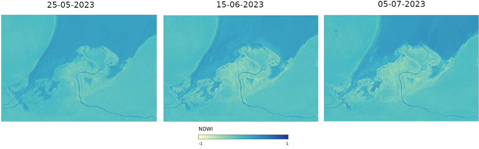
In this style of images,
dark blue means high probability of water occurrence, while
yellow means no water at all.
As you can see, mouth of the river starts to be more and more yellow with each month. We conclude that there barely is any water near the mouth of Syr Darya river. We can assume, that during the summer rivers lose lot of water. This can be happening because of
high temperatures, but also because
the people along the river are using more of its waters, to irrigate the fields.
Unfortunately, it means that the Aral Lake will still be dying and it is not impossible for us to witness its end – the end of what once used to be one of the biggest lakes on our planet.
What To Do Next
Interested to see additional examples of studying nature via satellite images?
Urban sprawl:
Floods:
Analyzing and monitoring floods using Python and Sentinel-2 satellite imagery on Creodias
Polluted air:
Processing Sentinel-5P data on air pollution using Jupyter Notebook on Creodias