Processing Sentinel-5P data on air pollution using Jupyter Notebook on CREODIAS

Prerequisites

No. 1 Hosting

You need a CREODIAS hosting account with access to the Horizon interface: https://horizon.cloudferro.com.

No. 2 Installing Jupyter Notebook

The code in this article runs on Jupyter Notebook and you can install it on your platform of choice by following the offical Jupyter Notebook install page.

One particular way of installing (and by no means being required to follow up this article), is to install it on Kubernetes cluster. If that is the case, this article will come handy:

Installing JupyterHub on Magnum Kubernetes Cluster in CREODIAS Cloud.

PART #1 - Download and prepare data

This notebook aims to present how to process Sentinel-5P data and prepare it for further analysis, using HARP, via CREODIAS platfrom.

In this notebook you will learn how to:

create a query via https://explore.creodias.eu/

upload data from eodata CREODIAS repository

read many of Sentinel-5P images (netCDF)

process Sentinel-5P images (tropospheric column of NO2 - NO2 TVCD) using HARP

create a single image which is going to be monthly average of NO2 TVCD (netcdf)

plot results

Datasets which are going to be used:

Sentinel-5P (product L2__NO2___) - 01.03.2023 - 31.03.2023; limited to Poland

Districts of Poland https://www.geoportal.gov.pl/dane/panstwowy-rejestr-granic

HARP https://atmospherictoolbox.org/harp/

Import libraries

import harp
import numpy as np
import matplotlib.pyplot as plt
import cartopy.crs as ccrs
import cartopy.io.img_tiles as cimgt
from cmcrameri import cm
import json, requests, os

Upload data using query generated by Data Explorer

Additionally, you can set time of analysis:

start	first day of analysed period
end	last day od analysed period

start = str("2023-03-01") #first day of the analysed period
end = str("2023-03-31")   #last day of the analysed period

#querry generated by Data Explorer
url = f"https://datahub.creodias.eu/odata/v1/Products?$filter=((ContentDate/Start ge {start}T00:00:00.000Z and ContentDate/Start le {end}T23:59:59.999Z) and (Online eq true) and (OData.CSC.Intersects(Footprint=geography'SRID=4326;POLYGON ((13.44866 55.702105, 24.616418 55.287061, 24.505406 48.582106, 13.359851 49.556626, 13.44866 55.702105))')) and (((((((Attributes/OData.CSC.StringAttribute/any(i0:i0/Name eq 'productType' and i0/Value eq 'L2__NO2___')))) and (((Attributes/OData.CSC.StringAttribute/any(i0:i0/Name eq 'processingMode' and i0/Value eq 'OFFL')))) and (Collection/Name eq 'SENTINEL-5P'))))))&$expand=Attributes&$top=1000"

#take a look on result url
"https://datahub.creodias.eu/odata/v1/Products?$filter=((ContentDate/Start ge 2023-03-01T00:00:00.000Z and ContentDate/Start le 2023-03-31T23:59:59.999Z) and (Online eq true) and (OData.CSC.Intersects(Footprint=geography'SRID=4326;POLYGON ((13.44866 55.702105, 24.616418 55.287061, 24.505406 48.582106, 13.359851 49.556626, 13.44866 55.702105))')) and (((((((Attributes/OData.CSC.StringAttribute/any(i0:i0/Name eq 'productType' and i0/Value eq 'L2__NO2___')))) and (((Attributes/OData.CSC.StringAttribute/any(i0:i0/Name eq 'processingMode' and i0/Value eq 'OFFL')))) and (Collection/Name eq 'SENTINEL-5P'))))))&$expand=Attributes&$top=1000"

Define lists of paths of files and files’ names

#get list of products (JSON)
products = json.loads(requests.get(url).text)

path_list = []                           #create an empty list to store the file names
for item in products['value']:
    path_list.append(item['S3Path'])     #append each S3Path (path) to the list
    print(item['S3Path'])                #print each S3Path (path) to the list

name_list = []                           #create an empty list to store the file names
for item in products['value']:
    name_list.append(item['Name'])       #append each Name (name) to the list
    print(item['Name'])                  #print each Name (name) to the list

/eodata/Sentinel-5P/TROPOMI/L2__NO2___/2023/03/29/S5P_OFFL_L2__NO2____20230329T113029_20230329T131159_28277_03_020500_20230331T035449
/eodata/Sentinel-5P/TROPOMI/L2__NO2___/2023/03/29/S5P_OFFL_L2__NO2____20230329T094858_20230329T113029_28276_03_020500_20230331T021341
/eodata/Sentinel-5P/TROPOMI/L2__NO2___/2023/03/10/S5P_OFFL_L2__NO2____20230310T104321_20230310T122451_28007_03_020400_20230312T025817
/eodata/Sentinel-5P/TROPOMI/L2__NO2___/2023/03/30/S5P_OFFL_L2__NO2____20230330T093006_20230330T111136_28290_03_020500_20230401T015114
/eodata/Sentinel-5P/TROPOMI/L2__NO2___/2023/03/07/S5P_OFFL_L2__NO2____20230307T114008_20230307T132138_27965_03_020400_20230309T040214
/eodata/Sentinel-5P/TROPOMI/L2__NO2___/2023/03/09/S5P_OFFL_L2__NO2____20230309T110217_20230309T124347_27993_03_020400_20230311T031357
/eodata/Sentinel-5P/TROPOMI/L2__NO2___/2023/03/20/S5P_OFFL_L2__NO2____20230320T091549_20230320T105720_28148_03_020500_20230322T012553
/eodata/Sentinel-5P/TROPOMI/L2__NO2___/2023/03/13/S5P_OFFL_L2__NO2____20230313T112803_20230313T130934_28050_03_020500_20230316T030602
/eodata/Sentinel-5P/TROPOMI/L2__NO2___/2023/03/02/S5P_OFFL_L2__NO2____20230302T113316_20230302T131447_27894_03_020400_20230304T041315
/eodata/Sentinel-5P/TROPOMI/L2__NO2___/2023/03/02/S5P_OFFL_L2__NO2____20230302T095146_20230302T113316_27893_03_020400_20230304T021515
/eodata/Sentinel-5P/TROPOMI/L2__NO2___/2023/03/05/S5P_OFFL_L2__NO2____20230305T085459_20230305T103629_27935_03_020400_20230307T011244
/eodata/Sentinel-5P/TROPOMI/L2__NO2___/2023/03/05/S5P_OFFL_L2__NO2____20230305T103629_20230305T121800_27936_03_020400_20230307T030702
/eodata/Sentinel-5P/TROPOMI/L2__NO2___/2023/03/08/S5P_OFFL_L2__NO2____20230308T093942_20230308T112112_27978_03_020400_20230310T015134
/eodata/Sentinel-5P/TROPOMI/L2__NO2___/2023/03/14/S5P_OFFL_L2__NO2____20230314T110908_20230314T125038_28064_03_020500_20230317T111227
/eodata/Sentinel-5P/TROPOMI/L2__NO2___/2023/03/08/S5P_OFFL_L2__NO2____20230308T112112_20230308T130243_27979_03_020400_20230310T033310
/eodata/Sentinel-5P/TROPOMI/L2__NO2___/2023/03/26/S5P_OFFL_L2__NO2____20230326T104536_20230326T122707_28234_03_020500_20230328T030428
/eodata/Sentinel-5P/TROPOMI/L2__NO2___/2023/03/26/S5P_OFFL_L2__NO2____20230326T090405_20230326T104536_28233_03_020500_20230328T011028
/eodata/Sentinel-5P/TROPOMI/L2__NO2___/2023/03/15/S5P_OFFL_L2__NO2____20230315T090841_20230315T105012_28077_03_020500_20230318T003027
/eodata/Sentinel-5P/TROPOMI/L2__NO2___/2023/03/19/S5P_OFFL_L2__NO2____20230319T093442_20230319T111612_28134_03_020500_20230321T014727
/eodata/Sentinel-5P/TROPOMI/L2__NO2___/2023/03/31/S5P_OFFL_L2__NO2____20230331T091113_20230331T105243_28304_03_020500_20230402T011756
/eodata/Sentinel-5P/TROPOMI/L2__NO2___/2023/03/31/S5P_OFFL_L2__NO2____20230331T105243_20230331T123414_28305_03_020500_20230402T031349
/eodata/Sentinel-5P/TROPOMI/L2__NO2___/2023/03/11/S5P_OFFL_L2__NO2____20230311T102425_20230311T120555_28021_03_020400_20230313T023618
/eodata/Sentinel-5P/TROPOMI/L2__NO2___/2023/03/04/S5P_OFFL_L2__NO2____20230304T091355_20230304T105525_27921_03_020400_20230306T013254
/eodata/Sentinel-5P/TROPOMI/L2__NO2___/2023/03/01/S5P_OFFL_L2__NO2____20230301T101042_20230301T115212_27879_03_020400_20230303T023224
/eodata/Sentinel-5P/TROPOMI/L2__NO2___/2023/03/28/S5P_OFFL_L2__NO2____20230328T114921_20230328T133052_28263_03_020500_20230330T042453
/eodata/Sentinel-5P/TROPOMI/L2__NO2___/2023/03/14/S5P_OFFL_L2__NO2____20230314T092737_20230314T110908_28063_03_020500_20230317T110733
/eodata/Sentinel-5P/TROPOMI/L2__NO2___/2023/03/28/S5P_OFFL_L2__NO2____20230328T100751_20230328T114921_28262_03_020500_20230330T023332
/eodata/Sentinel-5P/TROPOMI/L2__NO2___/2023/03/17/S5P_OFFL_L2__NO2____20230317T101226_20230317T115357_28106_03_020500_20230319T082226
/eodata/Sentinel-5P/TROPOMI/L2__NO2___/2023/03/17/S5P_OFFL_L2__NO2____20230317T083056_20230317T101226_28105_03_020500_20230319T062640
/eodata/Sentinel-5P/TROPOMI/L2__NO2___/2023/03/16/S5P_OFFL_L2__NO2____20230316T103118_20230316T121249_28092_03_020500_20230318T193655
/eodata/Sentinel-5P/TROPOMI/L2__NO2___/2023/03/27/S5P_OFFL_L2__NO2____20230327T084513_20230327T102644_28247_03_020500_20230329T004554
/eodata/Sentinel-5P/TROPOMI/L2__NO2___/2023/03/04/S5P_OFFL_L2__NO2____20230304T105525_20230304T123655_27922_03_020400_20230306T032707
/eodata/Sentinel-5P/TROPOMI/L2__NO2___/2023/03/12/S5P_OFFL_L2__NO2____20230312T082359_20230312T100529_28034_03_020500_20230315T154142
/eodata/Sentinel-5P/TROPOMI/L2__NO2___/2023/03/12/S5P_OFFL_L2__NO2____20230312T100529_20230312T114659_28035_03_020500_20230315T154412
/eodata/Sentinel-5P/TROPOMI/L2__NO2___/2023/03/12/S5P_OFFL_L2__NO2____20230312T114659_20230312T132830_28036_03_020500_20230315T155238
S5P_OFFL_L2__NO2____20230329T113029_20230329T131159_28277_03_020500_20230331T035449.nc
S5P_OFFL_L2__NO2____20230329T094858_20230329T113029_28276_03_020500_20230331T021341.nc
S5P_OFFL_L2__NO2____20230310T104321_20230310T122451_28007_03_020400_20230312T025817.nc
S5P_OFFL_L2__NO2____20230330T093006_20230330T111136_28290_03_020500_20230401T015114.nc
S5P_OFFL_L2__NO2____20230307T114008_20230307T132138_27965_03_020400_20230309T040214.nc
S5P_OFFL_L2__NO2____20230309T110217_20230309T124347_27993_03_020400_20230311T031357.nc
S5P_OFFL_L2__NO2____20230320T091549_20230320T105720_28148_03_020500_20230322T012553.nc
S5P_OFFL_L2__NO2____20230313T112803_20230313T130934_28050_03_020500_20230316T030602.nc
S5P_OFFL_L2__NO2____20230302T113316_20230302T131447_27894_03_020400_20230304T041315.nc
S5P_OFFL_L2__NO2____20230302T095146_20230302T113316_27893_03_020400_20230304T021515.nc
S5P_OFFL_L2__NO2____20230305T085459_20230305T103629_27935_03_020400_20230307T011244.nc
S5P_OFFL_L2__NO2____20230305T103629_20230305T121800_27936_03_020400_20230307T030702.nc
S5P_OFFL_L2__NO2____20230308T093942_20230308T112112_27978_03_020400_20230310T015134.nc
S5P_OFFL_L2__NO2____20230314T110908_20230314T125038_28064_03_020500_20230317T111227.nc
S5P_OFFL_L2__NO2____20230308T112112_20230308T130243_27979_03_020400_20230310T033310.nc
S5P_OFFL_L2__NO2____20230326T104536_20230326T122707_28234_03_020500_20230328T030428.nc
S5P_OFFL_L2__NO2____20230326T090405_20230326T104536_28233_03_020500_20230328T011028.nc
S5P_OFFL_L2__NO2____20230315T090841_20230315T105012_28077_03_020500_20230318T003027.nc
S5P_OFFL_L2__NO2____20230319T093442_20230319T111612_28134_03_020500_20230321T014727.nc
S5P_OFFL_L2__NO2____20230331T091113_20230331T105243_28304_03_020500_20230402T011756.nc
S5P_OFFL_L2__NO2____20230331T105243_20230331T123414_28305_03_020500_20230402T031349.nc
S5P_OFFL_L2__NO2____20230311T102425_20230311T120555_28021_03_020400_20230313T023618.nc
S5P_OFFL_L2__NO2____20230304T091355_20230304T105525_27921_03_020400_20230306T013254.nc
S5P_OFFL_L2__NO2____20230301T101042_20230301T115212_27879_03_020400_20230303T023224.nc
S5P_OFFL_L2__NO2____20230328T114921_20230328T133052_28263_03_020500_20230330T042453.nc
S5P_OFFL_L2__NO2____20230314T092737_20230314T110908_28063_03_020500_20230317T110733.nc
S5P_OFFL_L2__NO2____20230328T100751_20230328T114921_28262_03_020500_20230330T023332.nc
S5P_OFFL_L2__NO2____20230317T101226_20230317T115357_28106_03_020500_20230319T082226.nc
S5P_OFFL_L2__NO2____20230317T083056_20230317T101226_28105_03_020500_20230319T062640.nc
S5P_OFFL_L2__NO2____20230316T103118_20230316T121249_28092_03_020500_20230318T193655.nc
S5P_OFFL_L2__NO2____20230327T084513_20230327T102644_28247_03_020500_20230329T004554.nc
S5P_OFFL_L2__NO2____20230304T105525_20230304T123655_27922_03_020400_20230306T032707.nc
S5P_OFFL_L2__NO2____20230312T082359_20230312T100529_28034_03_020500_20230315T154142.nc
S5P_OFFL_L2__NO2____20230312T100529_20230312T114659_28035_03_020500_20230315T154412.nc
S5P_OFFL_L2__NO2____20230312T114659_20230312T132830_28036_03_020500_20230315T155238.nc

Create a list of merged paths and names of each image

separator = '/'                                    #set separator between path and name
result_list = [name + separator + path for name,   #create a list of merged paths and names for each image
               path in zip(path_list, name_list)]
print(result_list)

['/eodata/Sentinel-5P/TROPOMI/L2__NO2___/2023/03/29/S5P_OFFL_L2__NO2____20230329T113029_20230329T131159_28277_03_020500_20230331T035449/S5P_OFFL_L2__NO2____20230329T113029_20230329T131159_28277_03_020500_20230331T035449.nc', '/eodata/Sentinel-5P/TROPOMI/L2__NO2___/2023/03/29/S5P_OFFL_L2__NO2____20230329T094858_20230329T113029_28276_03_020500_20230331T021341/S5P_OFFL_L2__NO2____20230329T094858_20230329T113029_28276_03_020500_20230331T021341.nc', '/eodata/Sentinel-5P/TROPOMI/L2__NO2___/2023/03/10/S5P_OFFL_L2__NO2____20230310T104321_20230310T122451_28007_03_020400_20230312T025817/S5P_OFFL_L2__NO2____20230310T104321_20230310T122451_28007_03_020400_20230312T025817.nc', '/eodata/Sentinel-5P/TROPOMI/L2__NO2___/2023/03/30/S5P_OFFL_L2__NO2____20230330T093006_20230330T111136_28290_03_020500_20230401T015114/S5P_OFFL_L2__NO2____20230330T093006_20230330T111136_28290_03_020500_20230401T015114.nc', '/eodata/Sentinel-5P/TROPOMI/L2__NO2___/2023/03/07/S5P_OFFL_L2__NO2____20230307T114008_20230307T132138_27965_03_020400_20230309T040214/S5P_OFFL_L2__NO2____20230307T114008_20230307T132138_27965_03_020400_20230309T040214.nc', '/eodata/Sentinel-5P/TROPOMI/L2__NO2___/2023/03/09/S5P_OFFL_L2__NO2____20230309T110217_20230309T124347_27993_03_020400_20230311T031357/S5P_OFFL_L2__NO2____20230309T110217_20230309T124347_27993_03_020400_20230311T031357.nc', '/eodata/Sentinel-5P/TROPOMI/L2__NO2___/2023/03/20/S5P_OFFL_L2__NO2____20230320T091549_20230320T105720_28148_03_020500_20230322T012553/S5P_OFFL_L2__NO2____20230320T091549_20230320T105720_28148_03_020500_20230322T012553.nc', '/eodata/Sentinel-5P/TROPOMI/L2__NO2___/2023/03/13/S5P_OFFL_L2__NO2____20230313T112803_20230313T130934_28050_03_020500_20230316T030602/S5P_OFFL_L2__NO2____20230313T112803_20230313T130934_28050_03_020500_20230316T030602.nc', '/eodata/Sentinel-5P/TROPOMI/L2__NO2___/2023/03/02/S5P_OFFL_L2__NO2____20230302T113316_20230302T131447_27894_03_020400_20230304T041315/S5P_OFFL_L2__NO2____20230302T113316_20230302T131447_27894_03_020400_20230304T041315.nc', '/eodata/Sentinel-5P/TROPOMI/L2__NO2___/2023/03/02/S5P_OFFL_L2__NO2____20230302T095146_20230302T113316_27893_03_020400_20230304T021515/S5P_OFFL_L2__NO2____20230302T095146_20230302T113316_27893_03_020400_20230304T021515.nc', '/eodata/Sentinel-5P/TROPOMI/L2__NO2___/2023/03/05/S5P_OFFL_L2__NO2____20230305T085459_20230305T103629_27935_03_020400_20230307T011244/S5P_OFFL_L2__NO2____20230305T085459_20230305T103629_27935_03_020400_20230307T011244.nc', '/eodata/Sentinel-5P/TROPOMI/L2__NO2___/2023/03/05/S5P_OFFL_L2__NO2____20230305T103629_20230305T121800_27936_03_020400_20230307T030702/S5P_OFFL_L2__NO2____20230305T103629_20230305T121800_27936_03_020400_20230307T030702.nc', '/eodata/Sentinel-5P/TROPOMI/L2__NO2___/2023/03/08/S5P_OFFL_L2__NO2____20230308T093942_20230308T112112_27978_03_020400_20230310T015134/S5P_OFFL_L2__NO2____20230308T093942_20230308T112112_27978_03_020400_20230310T015134.nc', '/eodata/Sentinel-5P/TROPOMI/L2__NO2___/2023/03/14/S5P_OFFL_L2__NO2____20230314T110908_20230314T125038_28064_03_020500_20230317T111227/S5P_OFFL_L2__NO2____20230314T110908_20230314T125038_28064_03_020500_20230317T111227.nc', '/eodata/Sentinel-5P/TROPOMI/L2__NO2___/2023/03/08/S5P_OFFL_L2__NO2____20230308T112112_20230308T130243_27979_03_020400_20230310T033310/S5P_OFFL_L2__NO2____20230308T112112_20230308T130243_27979_03_020400_20230310T033310.nc', '/eodata/Sentinel-5P/TROPOMI/L2__NO2___/2023/03/26/S5P_OFFL_L2__NO2____20230326T104536_20230326T122707_28234_03_020500_20230328T030428/S5P_OFFL_L2__NO2____20230326T104536_20230326T122707_28234_03_020500_20230328T030428.nc', '/eodata/Sentinel-5P/TROPOMI/L2__NO2___/2023/03/26/S5P_OFFL_L2__NO2____20230326T090405_20230326T104536_28233_03_020500_20230328T011028/S5P_OFFL_L2__NO2____20230326T090405_20230326T104536_28233_03_020500_20230328T011028.nc', '/eodata/Sentinel-5P/TROPOMI/L2__NO2___/2023/03/15/S5P_OFFL_L2__NO2____20230315T090841_20230315T105012_28077_03_020500_20230318T003027/S5P_OFFL_L2__NO2____20230315T090841_20230315T105012_28077_03_020500_20230318T003027.nc', '/eodata/Sentinel-5P/TROPOMI/L2__NO2___/2023/03/19/S5P_OFFL_L2__NO2____20230319T093442_20230319T111612_28134_03_020500_20230321T014727/S5P_OFFL_L2__NO2____20230319T093442_20230319T111612_28134_03_020500_20230321T014727.nc', '/eodata/Sentinel-5P/TROPOMI/L2__NO2___/2023/03/31/S5P_OFFL_L2__NO2____20230331T091113_20230331T105243_28304_03_020500_20230402T011756/S5P_OFFL_L2__NO2____20230331T091113_20230331T105243_28304_03_020500_20230402T011756.nc', '/eodata/Sentinel-5P/TROPOMI/L2__NO2___/2023/03/31/S5P_OFFL_L2__NO2____20230331T105243_20230331T123414_28305_03_020500_20230402T031349/S5P_OFFL_L2__NO2____20230331T105243_20230331T123414_28305_03_020500_20230402T031349.nc', '/eodata/Sentinel-5P/TROPOMI/L2__NO2___/2023/03/11/S5P_OFFL_L2__NO2____20230311T102425_20230311T120555_28021_03_020400_20230313T023618/S5P_OFFL_L2__NO2____20230311T102425_20230311T120555_28021_03_020400_20230313T023618.nc', '/eodata/Sentinel-5P/TROPOMI/L2__NO2___/2023/03/04/S5P_OFFL_L2__NO2____20230304T091355_20230304T105525_27921_03_020400_20230306T013254/S5P_OFFL_L2__NO2____20230304T091355_20230304T105525_27921_03_020400_20230306T013254.nc', '/eodata/Sentinel-5P/TROPOMI/L2__NO2___/2023/03/01/S5P_OFFL_L2__NO2____20230301T101042_20230301T115212_27879_03_020400_20230303T023224/S5P_OFFL_L2__NO2____20230301T101042_20230301T115212_27879_03_020400_20230303T023224.nc', '/eodata/Sentinel-5P/TROPOMI/L2__NO2___/2023/03/28/S5P_OFFL_L2__NO2____20230328T114921_20230328T133052_28263_03_020500_20230330T042453/S5P_OFFL_L2__NO2____20230328T114921_20230328T133052_28263_03_020500_20230330T042453.nc', '/eodata/Sentinel-5P/TROPOMI/L2__NO2___/2023/03/14/S5P_OFFL_L2__NO2____20230314T092737_20230314T110908_28063_03_020500_20230317T110733/S5P_OFFL_L2__NO2____20230314T092737_20230314T110908_28063_03_020500_20230317T110733.nc', '/eodata/Sentinel-5P/TROPOMI/L2__NO2___/2023/03/28/S5P_OFFL_L2__NO2____20230328T100751_20230328T114921_28262_03_020500_20230330T023332/S5P_OFFL_L2__NO2____20230328T100751_20230328T114921_28262_03_020500_20230330T023332.nc', '/eodata/Sentinel-5P/TROPOMI/L2__NO2___/2023/03/17/S5P_OFFL_L2__NO2____20230317T101226_20230317T115357_28106_03_020500_20230319T082226/S5P_OFFL_L2__NO2____20230317T101226_20230317T115357_28106_03_020500_20230319T082226.nc', '/eodata/Sentinel-5P/TROPOMI/L2__NO2___/2023/03/17/S5P_OFFL_L2__NO2____20230317T083056_20230317T101226_28105_03_020500_20230319T062640/S5P_OFFL_L2__NO2____20230317T083056_20230317T101226_28105_03_020500_20230319T062640.nc', '/eodata/Sentinel-5P/TROPOMI/L2__NO2___/2023/03/16/S5P_OFFL_L2__NO2____20230316T103118_20230316T121249_28092_03_020500_20230318T193655/S5P_OFFL_L2__NO2____20230316T103118_20230316T121249_28092_03_020500_20230318T193655.nc', '/eodata/Sentinel-5P/TROPOMI/L2__NO2___/2023/03/27/S5P_OFFL_L2__NO2____20230327T084513_20230327T102644_28247_03_020500_20230329T004554/S5P_OFFL_L2__NO2____20230327T084513_20230327T102644_28247_03_020500_20230329T004554.nc', '/eodata/Sentinel-5P/TROPOMI/L2__NO2___/2023/03/04/S5P_OFFL_L2__NO2____20230304T105525_20230304T123655_27922_03_020400_20230306T032707/S5P_OFFL_L2__NO2____20230304T105525_20230304T123655_27922_03_020400_20230306T032707.nc', '/eodata/Sentinel-5P/TROPOMI/L2__NO2___/2023/03/12/S5P_OFFL_L2__NO2____20230312T082359_20230312T100529_28034_03_020500_20230315T154142/S5P_OFFL_L2__NO2____20230312T082359_20230312T100529_28034_03_020500_20230315T154142.nc', '/eodata/Sentinel-5P/TROPOMI/L2__NO2___/2023/03/12/S5P_OFFL_L2__NO2____20230312T100529_20230312T114659_28035_03_020500_20230315T154412/S5P_OFFL_L2__NO2____20230312T100529_20230312T114659_28035_03_020500_20230315T154412.nc', '/eodata/Sentinel-5P/TROPOMI/L2__NO2___/2023/03/12/S5P_OFFL_L2__NO2____20230312T114659_20230312T132830_28036_03_020500_20230315T155238/S5P_OFFL_L2__NO2____20230312T114659_20230312T132830_28036_03_020500_20230315T155238.nc']

Using HARP - Atmospheric Toolbox

Using HARP - bin_spatial

“bin_spatial(A,S,SR,B,W,SR)”

A - is the number of latitude edge points, calculates as follows: (N latitude of AoI (55) - S latitude of AOI (49) / C (0.01)) + 1

S - is the latitude offset at which to start the grid (S)

SR - is the spatial resolution expressed in degrees

B - is the number of longitude edge points, calculates as follows: (E longitude of AoI (25) - W longitude of AOI (14) / C (0.01)) + 1

W - is the longitude offset at which to start the grid (W)

SR - is the spatial resolution expressed in degrees

N = 55.00
S = 49.00
W = 14.00
E = 25.00

SR = 0.01

A = (N-S)/SR + 1
B = (E-W)/SR + 1

operations = ";".join([
    "tropospheric_NO2_column_number_density_validity>75",             #keep pixels wich qa_value > 0.75
    "derive(surface_wind_speed {time} [m/s])",                        #get surafe wind speed expressed in [m/s]
    "surface_wind_speed<5",                                           #keep pixels wich wind_spped < 5 [m/s]
    #keep variables defined below
    "keep(latitude_bounds,longitude_bounds,datetime_start,datetime_length,tropospheric_NO2_column_number_density, surface_wind_speed)",
    "derive(datetime_start {time} [days since 2000-01-01])",          #get start time of the acquisition
    "derive(datetime_stop {time}[days since 2000-01-01])",            #get end time of the acquisition
    "exclude(datetime_length)",                                       #exclude datetime lenght
    f"bin_spatial({int(A)},{int(S)},{float(SR)},{int(B)},{int(W)},{float(SR)})",                       #define bin spatial (details below)
    "derive(tropospheric_NO2_column_number_density [Pmolec/cm2])",    #convert the NO2 units to 10^15 molec/cm^2
    "derive(latitude {latitude})",                                    #get latitude
    "derive(longitude {longitude})",                                  #get longitude
    "count>0"
])

Operations for temporal averaging

reduce_operations=";".join([
    "squash(time, (latitude, longitude, latitude_bounds, longitude_bounds))",
    "bin()"
])

Create new image - average NO2 pollution over defined area in specific period

mean_no2 = harp.import_product(result_list, operations, reduce_operations=reduce_operations)

Import and write new created image as a netcdf named “mean_no2_2023_03.nc”

harp.export_product(mean_no2, 'mean_no2_2023_03.nc') #name of varibale, name of new created file with extension

Define variable, longitude, latitude and colormap which are going to be visualized

#select NO2 pollution
no2 = mean_no2.tropospheric_NO2_column_number_density.data
#select desription (name) of variable
no2_description = mean_no2.tropospheric_NO2_column_number_density.description
#select units of variable
no2_units = mean_no2.tropospheric_NO2_column_number_density.unit

#define cooridantes grid
gridlat = np.append(mean_no2.latitude_bounds.data[:,0], mean_no2.latitude_bounds.data[-1,1])
gridlon = np.append(mean_no2.longitude_bounds.data[:,0], mean_no2.longitude_bounds.data[-1,1])

#define legend
colortable = cm.roma_r  #colors
vmin = 0                #min value
vmax = 10               #max value

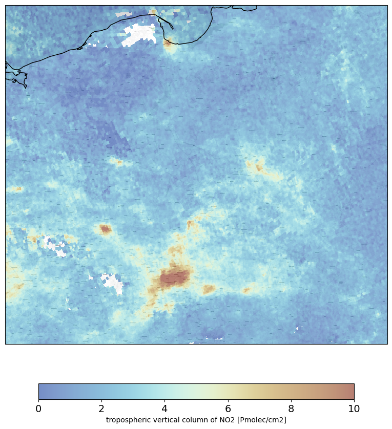
Create a visualization

boundaries=[14, 25, 49, 55.0]                       #define boundaries (W, E, S, N)

fig = plt.figure(figsize=(10,10))                   #size of the figure
bmap=cimgt.Stamen(style='toner-lite')               #set background
ax = plt.axes(projection=bmap.crs)
ax.set_extent(boundaries,crs = ccrs.PlateCarree())

zoom = 10
ax.add_image(bmap, zoom)

img = plt.pcolormesh(gridlon, gridlat,
                     no2[0,:,:], vmin=vmin, vmax=vmax,
                     cmap=colortable,
                     transform=ccrs.PlateCarree(),alpha = 0.55)
ax.coastlines()

cbar = fig.colorbar(img, ax=ax,orientation='horizontal', fraction=0.04, pad=0.1)
cbar.set_label(f'{no2_description} [{no2_units}]')
cbar.ax.tick_params(labelsize=14)

plt.show()

PART #2 - Conversion and zonal statistics

This part aims to present how to convert Sentinel-5P netCDF data into GeoTiff image and calculate zonal statistics, via CREODIAS platfrom

In this part you will learn how to:

convert netCDF into GeoTiff

calculate mean tropospheric column of NO2 (NO2 TVCD) for each Poland’s district and save results as a new-created shapefile

plot netCDF - NO2 TVCD values, for area of interest

plot mean NO2 TVCD for each Poland’s district as a choropleth

export new-created choropleth to a .jpg

put mean NO2 TVCD for each Poland’s district to a data frame and export it as a .csv

Datasets which are going to be used:

mean_no2_2023_03.nc - netCDF created by HARP processor

districts of Poland https://www.geoportal.gov.pl/dane/panstwowy-rejestr-granic

Import libraries
#Import libraries

import pandas as pd
import geopandas as gpd
import xarray as xr
import numpy as np
import os
import matplotlib.pyplot as plt
from mpl_toolkits.basemap import Basemap
import rasterstats
import rasterio
import rioxarray
from rasterio.plot import show
from rasterio.transform import from_origin

Export image as a GeoTiff and show results

#open the netcdf file
r1 = xr.open_dataset('mean_no2_2023_03.nc')

#extract the tropospheric_NO2_column_number_density variable
no2 = r1['tropospheric_NO2_column_number_density'].values[0,:,:]
#reverse order of the values within the array
no2 = no2[::-1]

#get the latitude and longitude coordinates
y = r1['latitude'].values
x = r1['longitude'].values

#reverse the latitude and longitude coordinates
y = y[::-1]
x = x[::-1]

#convert the DataArray to a rioxarray DataArray
da = xr.DataArray(no2,
                  coords={'y': y, 'x': x},
                  dims=('y', 'x'),
                  attrs={'crs': 'EPSG:4326'})

#save the rioxarray DataArray to a GeoTIFF file with CRS 4326
da.rio.to_raster('mean_no2_2023_03.tif', crs='EPSG:4326')

#open new-crtead raster
src = rasterio.open("mean_no2_2023_03.tif")

#plot the new-created raster
show(src)

Calculate mean NO2 TVCD for each Poland’s district and save results as a new-created shapefile

# -*- coding: utf-8 -*-
#read shapefile of districts in Poland
shapefile_path = 'poland_pow.shp'
poland_pow = gpd.read_file(shapefile_path)

#define the affine transformation (pixel size and coordinates of the top-left corner of the raster)
affine = rasterio.transform.from_bounds(min(x), min(y),
                                        max(x), max(y),
                                        len(da.x), len(da.y))

#loop over the polygons in the poland_pow GeoDataFrame and calculate the mean NO2 TVCD for each polygon
mean_no2 = []
for i, row in poland_pow.iterrows():
    #extract the geometry of the polygon
    geometry = row.geometry
    #calculate the mean NO2 TVCD for the polygon
    mean_no2p = rasterstats.zonal_stats(geometry,
                                        da.values,
                                        affine=affine,
                                        nodata=-999,
                                        stats=['mean'],
                                        nan='ignore')[0]['mean']
    #add the mean NO2 TVCD value to the poland_pow GeoDataFrame properties
    poland_pow.loc[i, 'mean_no2'] = mean_no2p

#encode names of districts to UTF-8
poland_pow['JPT_NAZWA_'] = poland_pow['JPT_NAZWA_'].apply(lambda x: x.encode('latin-1').decode('utf-8'))
#save the GeoDataFrame with the mean NO2 TVCD values to a new shapefile
poland_pow.to_file('nuts_2023_03.shp', encoding='utf-8')

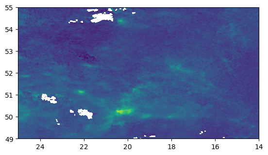
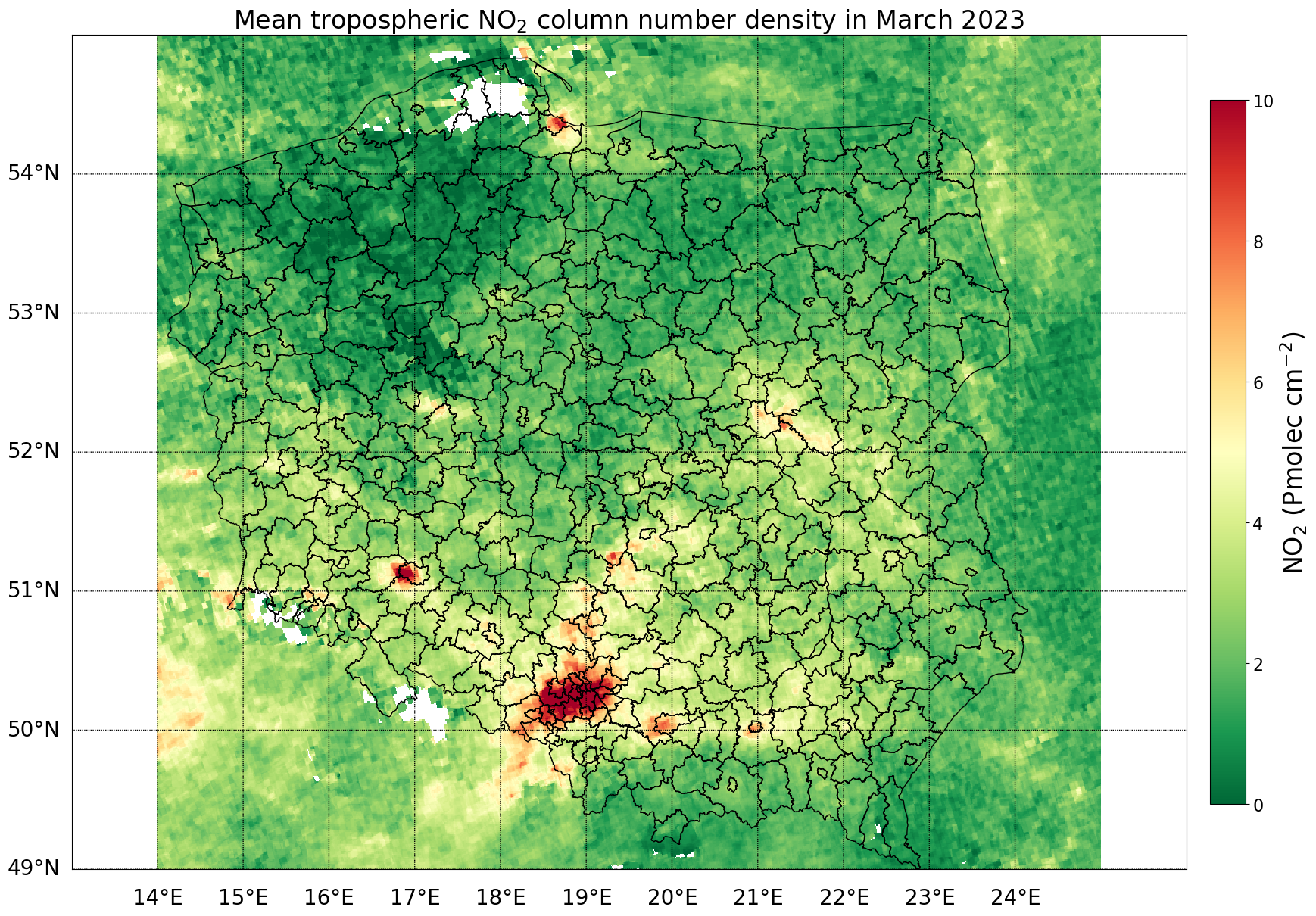
Plot netCDF - NO2 TVCD values, for area of interest - Poland

#open the netCDF file
nc_file = xr.open_dataset('mean_no2_2023_03.nc')

#read the tropospheric_NO2_column_number_density variable
no2_tvcd = nc_file['tropospheric_NO2_column_number_density'].values[0,:,]

#get the latitude and longitude coordinates from nc_file
lat = nc_file['latitude'].values
lon = nc_file['longitude'].values

#create the figure and Basemap instance
fig = plt.figure(figsize=(20,20))

#create a basemap with the desired projection and latitude/longitude bounds - Poland
m = Basemap(projection='cyl', llcrnrlat=49, urcrnrlat=55,
            llcrnrlon=13, urcrnrlon=26, resolution='c')

#plot NO2 TVCD on basemap
x, y = m(lon, lat)
m.pcolormesh(x, y, no2_tvcd, cmap='RdYlGn_r', vmin=0, vmax=10)

#add coordinates grid
m.drawparallels(np.arange(49, 55, 1), labels=[1,0,0,0], fontsize=20)
m.drawmeridians(np.arange(14, 25, 1), labels=[0,0,0,1], fontsize=20)

#read shapefile of districts in Poland
shapefile_path = 'poland_pow.shp'               #define path
poland_nuts = gpd.read_file(shapefile_path)     #read file containing districts of Poland

#plot districts on map
poland_nuts.plot(ax=plt.gca(), facecolor='none', edgecolor='black', linewidth=1)

#add colorbar
cbar = plt.colorbar(fraction=0.03, pad=0.02)
cbar.ax.set_ylabel('NO$_2$ (Pmolec cm$^{-2}$)', fontsize=24)
cbar.ax.tick_params(labelsize=16)

#plot title
plt.title('Mean tropospheric NO$_2$ column number density in March 2023', fontsize=24)

#show plot
plt.show()

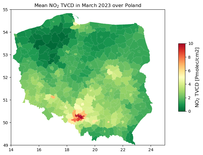
Plot mean NO2 TVCD for each Poland’s district - create choropleth

#read shapefile of NUTS3 regions in Poland
shapefile_path = 'nuts_2023_03.shp'          #define path
poland_nuts = gpd.read_file(shapefile_path)  #read file containing districts of Poland

#create a figure
fig, ax1 = plt.subplots(ncols=1, figsize=(12, 6))

#plot choropleth based on mean NO2 TVCD iver Poland
poland_nuts.plot(column='mean_no2',                  #mean_no2 is a column contains mean NO2 TVCD for each polygon
                 cmap='RdYlGn_r', ax=ax1)            #cmap - color ramp from green to red
ax1.set_xlim(14, 25)                                 #W-E extent of Poland
ax1.set_ylim(49, 55)                                 #S-N extent of Poland
ax1.set_title('Mean NO$_2$ TVCD in March 2023 over Poland')    #title of plot

#add a colorbar reffering to the the NO2 TVCD
vmin, vmax = [0, 10]                           #min and max value on colorbar
cbar = plt.cm.ScalarMappable(cmap='RdYlGn_r', norm=plt.Normalize(vmin=vmin, vmax=vmax))
plt.colorbar(cbar, ax=ax1, shrink=0.5, aspect=10).set_label('NO$_2$ TVCD [Pmolec/cm2]', fontsize=12)

#show the plot
plt.show()

Export image of mean NO2 TVCD for each Poland’s district to a .jpg

#save a plot as a .jpg
fig.savefig('POLAND_NO2_2023_03.jpg', dpi=300)

Put mean NO2 TVCD for each Poland’s district to a data frame

#get the mean NO2 TVCD values for each polygon in the Poland shapefile and round to two decimal places
no2_means = round(poland_nuts['mean_no2'],2)

#create a Pandas DataFrame with the mean NO2 TVCD values and their corresponding polygon names
NO2_df = pd.DataFrame({'Polygon': poland_nuts['JPT_NAZWA_'], 'Mean NO2': no2_means})

#sort the Poland's districts in descending order by the mean NO2 values values
NO2_df = NO2_df.sort_values(by='Mean NO2', ascending=False)

#print the DataFrame
print(NO2_df)

                         Polygon  Mean NO2
            powiat Katowice     10.76
         powiat Ruda Śląska     10.70
      powiat Świętochłowice     10.66
             powiat Chorzów     10.64
 powiat Siemianowice Śląskie     10.29
..                           ...       ...
          powiat chodzieski      0.52
            powiat obornicki      0.51
           powiat chojnicki      0.48
           powiat złotowski      0.42
             powiat drawski      0.36

[380 rows x 2 columns]

Export mean NO2 TVCD for each Poland’s district to a .csv file

NO2_df.to_csv('NO2_df.csv')