MODIS land cover deforestation analysis in Brazil using Jupyter Notebook on Creodias

Introduction

This article shows how to analyze long-term land cover change in the Brazilian Amazon by using a Jupyter Notebook on Creodias. The example uses the MODIS MCD12Q1 land cover product for the period from 2001 to 2024 and focuses on a region in the state of Pará, Brazil.

The workflow searches the CREODIAS OData catalogue, resolves the matching MODIS products, downloads the required HDF4 files from S3 to a local cache, and processes the LC_Type1 scientific dataset. The result is a set of charts and an animation showing how forest and non-forest land cover classes changed over time.

Unlike the fire and snow examples in this series, this workflow uses S3 access rather than direct /eodata filesystem access. This makes it suitable for environments where the notebook has network access and valid S3 credentials.

Overview

The notebook processes the MODIS MCD12Q1 product, which provides annual land cover classification at 500 m resolution. The analysis focuses on the IGBP classification layer LC_Type1.

The selected area is a rectangular region in Pará:

Boundary	Value
Minimum longitude	-53.0
Maximum longitude	-48.0
Minimum latitude	-6.0
Maximum latitude	-2.0

The workflow focuses on the land-cover classes most relevant to deforestation analysis:

IGBP class	Meaning
2	Evergreen Broadleaf Forest
8	Woody Savannas
9	Savannas
10	Grasslands
17	Water Bodies

What you will do

In this article, you will:

• prepare a Python environment inside a Jupyter Notebook,

• define an area of interest in the Brazilian Amazon,

• search the CREODIAS OData catalogue for MODIS land cover products,

• identify the matching MODIS tile and date range,

• download HDF4 files from S3 into a local cache,

• read the LC_Type1 land cover layer,

• calculate land cover statistics by year,

• create an animated land cover map,

• plot land cover composition and forest-area change over time.

Prerequisites

Before starting, make sure that the following requirements are met.

No. 1 Hosting

You need a Creodias hosting account with access to the Horizon interface:

https://horizon.cloudferro.com/auth/login/?next=/

No. 2 Installing Jupyter Notebook

The code in this article runs in Jupyter Notebook. You can install it on your platform of choice by following the official Jupyter Notebook installation page.

One possible way to run Jupyter Notebook is to install it on a Kubernetes cluster. This is not required for completing this article, but the following article may be useful if you choose that setup:

Installing JupyterHub on Magnum Kubernetes Cluster in Creodias

No. 3 Access to EODATA through S3

The notebook searches the CREODIAS catalogue and downloads selected MODIS files from S3 into a local cache. Make sure that you have valid S3 credentials and that your environment can access the EODATA S3 endpoint.

The S3 access articles are the most important for this workflow. The catalogue article is useful for understanding the OData search step, where the notebook selects products before downloading the matching HDF4 files.

Depending on how your environment is configured, you may need one of the following articles:

• How to access EODATA using S3 protocol on Creodias

• How to access EODATA using boto3 on Creodias

• How to download EODATA file using boto3 on Creodias

• EOData Catalogue API Manual on Creodias

No. 4 Notebook file

This article is accompanied by a ready-to-run Jupyter Notebook.

Download the notebook before running the workflow:

• Download the notebook

The notebook defines the area of interest directly in the code, so no local GeoPackage file is required for this article.

Required files

Only the notebook file is required for this workflow.

The notebook creates a local cache directory for downloaded MODIS HDF4 files. If you run the notebook again, files that already exist in the cache are reused and are not downloaded a second time.

Step 1. Install dependencies

The notebook uses Python packages for OData catalogue access, S3 download, HDF4 reading, image generation, plotting, and statistics.

Run the following cell at the beginning of the notebook:

import importlib, subprocess, sys

pkgs = [
    "pyhdf",
    "boto3",
    "matplotlib",
    "numpy",
    "scipy",
    "pillow",
    "requests",
]

missing = [p for p in pkgs if importlib.util.find_spec(p) is None]

if missing:
    subprocess.check_call([sys.executable, "-m", "pip", "install", "-q"] + missing)

The packages are used as follows:

Package	Purpose
requests	Sends OData catalogue requests.
boto3	Lists and downloads MODIS files from S3.
pyhdf	Reads HDF4 files produced by MODIS.
numpy and scipy	Support numerical processing and smoothing.
matplotlib	Creates static charts.
pillow	Builds animated GIF output.

Step 2. Import libraries and configure S3 access

Import the required libraries, configure the local cache, and prepare the S3 client.

import os
import gc
import time
import requests
import boto3
import numpy as np
import matplotlib.pyplot as plt

from pyhdf.SD import SD, SDC
from datetime import datetime
from collections import defaultdict
from concurrent.futures import ThreadPoolExecutor, as_completed
from IPython.display import HTML, display, clear_output
from PIL import Image
from scipy.signal import savgol_filter
from pathlib import Path

CACHE_DIR = Path("modis_cache_mcd12q1")
CACHE_DIR.mkdir(exist_ok=True)

S3_ENDPOINT = "https://eodata.cloudferro.com"

ACCESS_KEY = "replace-with-your-access-key"
SECRET_KEY = "replace-with-your-secret-key"

s3 = boto3.client(
    "s3",
    endpoint_url=S3_ENDPOINT,
    aws_access_key_id=ACCESS_KEY,
    aws_secret_access_key=SECRET_KEY,
)

Replace the placeholder credentials with your own S3 credentials before running the notebook.

Step 3. Define the area of interest and MODIS classes

The area of interest is defined directly in the notebook as a bounding box over Pará, Brazil.

MAX_WORKERS = min(8, os.cpu_count() or 4)
LAYER = "LC_Type1"

AOI_MINX, AOI_MAXX = -53.0, -48.0
AOI_MINY, AOI_MAXY = -6.0, -2.0

FOREST_CLS = 2
AOI_CLS = [2, 8, 9, 10, 17]

IGBP = {
    2: ("#1A8C1A", "Evergreen Broadleaf Forest"),
    8: ("#9ACD32", "Woody Savannas"),
    9: ("#BDB76B", "Savannas"),
    10: ("#90EE90", "Grasslands"),
    13: ("#FF4500", "Urban and Built-up"),
    17: ("#1E90FF", "Water Bodies"),
}

base_colors = ["#cccccc"] * 18
base_colors[0] = "#000000"

for cls, (color, label) in IGBP.items():
    base_colors[cls] = color

print("ready")
print(f"AOI: lon [{AOI_MINX}, {AOI_MAXX}], lat [{AOI_MINY}, {AOI_MAXY}]")
print(f"Layer: {LAYER}")

The class 2, Evergreen Broadleaf Forest, is the main class used for forest area tracking.

Step 4. Search the OData catalogue

The notebook searches the CREODIAS OData catalogue for MODIS MCD12Q1 products.

ODATA_BASE = "https://datahub.creodias.eu/odata/v1/Products"

aoi_wkt = (
    f"POLYGON(("
    f"{AOI_MINX} {AOI_MINY},"
    f"{AOI_MAXX} {AOI_MINY},"
    f"{AOI_MAXX} {AOI_MAXY},"
    f"{AOI_MINX} {AOI_MAXY},"
    f"{AOI_MINX} {AOI_MINY}"
    f"))"
)

odata_filter = (
    "Collection/Name eq 'TERRAAQUA'"
    " and contains(Name,'MCD12Q1')"
    " and contains(Name,'h13v09')"
    " and ContentDate/Start gt 2000-01-01T00:00:00.000Z"
    " and ContentDate/Start lt 2025-01-01T00:00:00.000Z"
    f" and OData.CSC.Intersects(area=geography'SRID=4326;{aoi_wkt}')"
)

def fetch_all_pages(odata_filter):
    products = []
    skip = 0
    page_size = 100

    while True:
        params = {
            "$filter": odata_filter,
            "$orderby": "ContentDate/Start asc",
            "$top": page_size,
            "$skip": skip,
            "$expand": "Locations",
        }

        response = requests.get(ODATA_BASE, params=params, timeout=60)
        response.raise_for_status()

        page = response.json().get("value", [])
        products.extend(page)

        if len(page) < page_size:
            break

        skip += page_size

    return products

products = fetch_all_pages(odata_filter)

print(f"Products found: {len(products)}")

if products:
    print(
        f"Date range: "
        f"{products[0]['ContentDate']['Start'][:10]} -> "
        f"{products[-1]['ContentDate']['Start'][:10]}"
    )

The query limits the result to MODIS tile h13v09, product MCD12Q1, and the selected date range.

Step 5. Download and process scenes

For each product, the notebook:

1. reads the S3 path from the OData metadata,

2. lists S3 objects under the product prefix,

3. finds the HDF4 file,

4. downloads it into the local cache if needed,

5. opens the LC_Type1 layer,

6. clips the tile to the area of interest,

7. counts pixels in each IGBP land-cover class.

Define helper functions for S3 path handling and HDF4 processing:

def s3path_from_product(product):
    """Return the S3 path from product locations."""
    for loc in product.get("Locations", []):
        if loc.get("FormatType") == "Extracted" and loc.get("S3Path"):
            return loc["S3Path"]

    for loc in product.get("Locations", []):
        if loc.get("S3Path"):
            return loc["S3Path"]

    return None

def find_hdf_key(bucket, prefix):
    """Return the first HDF file under the given S3 prefix."""
    response = s3.list_objects_v2(Bucket=bucket, Prefix=prefix)

    for obj in response.get("Contents", []):
        key = obj["Key"]

        if key.lower().endswith(".hdf"):
            return key

    return None

def download_product(product):
    """Download one MODIS HDF file to the local cache."""
    s3_path = s3path_from_product(product)

    if not s3_path:
        return None

    path = s3_path.removeprefix("s3:/").lstrip("/")
    bucket, prefix = path.split("/", 1)

    hdf_key = find_hdf_key(bucket, prefix)

    if not hdf_key:
        return None

    local_path = CACHE_DIR / os.path.basename(hdf_key)

    if not local_path.exists():
        s3.download_file(bucket, hdf_key, str(local_path))

    return local_path

Define a function that reads and summarizes one HDF file:

def process_product(product):
    """Download one product if needed, read LC_Type1, and count classes."""
    hdf = sds = None

    try:
        local_path = download_product(product)

        if local_path is None:
            return None

        hdf = SD(str(local_path), SDC.READ)
        sds = hdf.select(LAYER)

        arr = sds[:].astype(np.uint8)

        # MCD12Q1 tile size is 2400 x 2400.
        h, w = arr.shape

        col0 = max(0, min(w, int((AOI_MINX - (-60)) / 10 * w)))
        col1 = max(0, min(w, int((AOI_MAXX - (-60)) / 10 * w)))
        row0 = max(0, min(h, int((0 - AOI_MAXY) / 10 * h)))
        row1 = max(0, min(h, int((0 - AOI_MINY) / 10 * h)))

        clipped = arr[row0:row1, col0:col1]

        hist = {
            cls: int(np.sum(clipped == cls))
            for cls in range(1, 18)
        }

        valid_px = int(np.sum((clipped >= 1) & (clipped <= 17)))

        dt = datetime.fromisoformat(
            product["ContentDate"]["Start"].replace("Z", "+00:00")
        )

        return {
            "dt": dt,
            "year": dt.year,
            "hist": hist,
            "valid_px": valid_px,
            "arr": clipped,
        }

    except Exception:
        return None

    finally:
        try:
            if sds:
                sds.endaccess()
        except Exception:
            pass

        try:
            if hdf:
                hdf.end()
        except Exception:
            pass

Process all products:

results = []
processed = 0
total = len(products)
t_start = datetime.now()

with ThreadPoolExecutor(max_workers=MAX_WORKERS) as executor:
    futures = {executor.submit(process_product, product): product for product in products}

    for future in as_completed(futures):
        processed += 1
        result = future.result()

        if result is not None:
            results.append(result)

        pct = processed / total if total else 0
        bar = "█" * int(pct * 30) + "░" * (30 - int(pct * 30))

        clear_output(wait=True)
        print(f"[{bar}] {processed}/{total} ({pct * 100:.1f}%)")

        if processed % 20 == 0:
            gc.collect()

results = sorted(results, key=lambda r: r["dt"])

print(f"Done - {len(results)} valid yearly products")

The resulting list contains one processed land-cover record per available year.

Step 6. Create an animated land cover map

The notebook can render one map per year and combine the frames into an animated GIF. Each frame shows the spatial distribution of land-cover classes across the area of interest.

frames = []
years_unique = sorted({r["year"] for r in results})

for year in years_unique:
    year_results = [r for r in results if r["year"] == year]

    if not year_results:
        continue

    arr = year_results[0]["arr"]

    rgb = np.zeros((*arr.shape, 3), dtype=np.uint8)

    for cls, (color, label) in IGBP.items():
        hex_color = color.lstrip("#")
        rgb_color = tuple(int(hex_color[i:i + 2], 16) for i in (0, 2, 4))
        rgb[arr == cls] = rgb_color

    fig, ax = plt.subplots(figsize=(6, 5))
    ax.imshow(rgb)
    ax.set_title(f"MODIS land cover - Pará, Brazil ({year})")
    ax.axis("off")

    fig.canvas.draw()

    frame = np.frombuffer(fig.canvas.tostring_rgb(), dtype=np.uint8)
    frame = frame.reshape(fig.canvas.get_width_height()[::-1] + (3,))
    frames.append(Image.fromarray(frame))

    plt.close(fig)

if frames:
    frames[0].save(
        "modis_landcover_brazil.gif",
        save_all=True,
        append_images=frames[1:],
        duration=700,
        loop=0,
    )

Animated MODIS land cover map for the selected area in Pará, Brazil.

The animation is useful for quickly checking whether the spatial pattern changes as expected before moving to numerical summaries.

Step 7. Build aggregate time series

The next step aggregates land-cover classes by year and converts pixel counts to square kilometres.

year_hist = defaultdict(lambda: defaultdict(int))
year_valid = defaultdict(int)

for r in results:
    for cls, count in r["hist"].items():
        year_hist[r["year"]][cls] += count

    year_valid[r["year"]] += r["valid_px"]

years = sorted(year_hist.keys())

def px_to_km2(px):
    return px * 500 * 500 / 1_000_000

def pct(year, cls):
    if not year_valid[year]:
        return 0

    return year_hist[year][cls] / year_valid[year] * 100

forest_km2 = [px_to_km2(year_hist[y][FOREST_CLS]) for y in years]
forest_delta = [value - forest_km2[0] for value in forest_km2]

gainers = []

for cls in AOI_CLS:
    if cls == FOREST_CLS:
        continue

    start = year_hist[years[0]][cls]
    end = year_hist[years[-1]][cls]

    if end > start:
        gainers.append(cls)

print(f"Years in analysis: {years[0]}-{years[-1]}")
print(f"Gainer classes: {gainers}")

The gainers list contains land-cover classes whose area increased between the first and last year.

Step 8. Plot land cover composition over time

A stacked area chart shows how the share of each selected land-cover class changed over time.

stack_classes = [FOREST_CLS] + gainers

if 17 not in stack_classes:
    stack_classes.append(17)

stack_data = [
    [pct(year, cls) for year in years]
    for cls in stack_classes
]

stack_labels = [IGBP[cls][1] for cls in stack_classes]
stack_colors = [IGBP[cls][0] for cls in stack_classes]

fig, ax = plt.subplots(figsize=(13, 4))

ax.stackplot(
    years,
    stack_data,
    labels=stack_labels,
    colors=stack_colors,
    alpha=0.85,
)

ax.set_xlim(years[0], years[-1])
ax.set_ylim(0, 100)
ax.set_title("Land cover composition over time")
ax.set_ylabel("Share (%)")
ax.legend(loc="upper left", fontsize=8)
ax.grid(True, alpha=0.25)

fig.tight_layout()
plt.show()

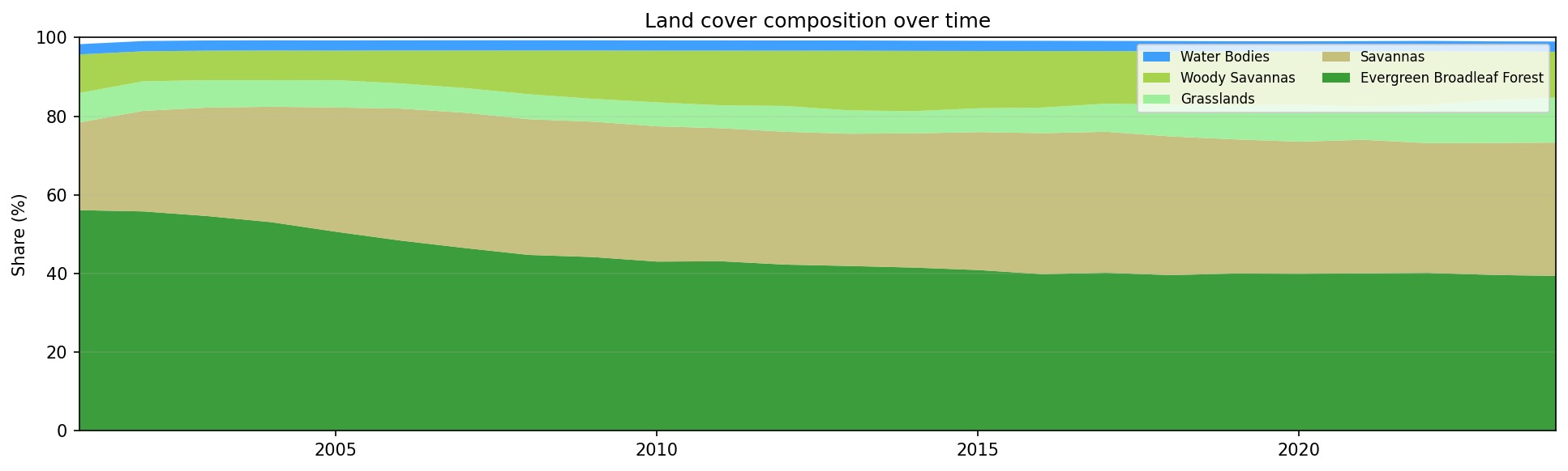
Land cover composition in the selected area of Pará, Brazil, from 2001 to 2024.

A shrinking forest band, combined with growing savanna or grassland classes, is a typical visual signature of deforestation and land-cover transition.

Step 9. Plot net area change

The next chart shows area change relative to the first available year.

fig, ax = plt.subplots(figsize=(13, 4))

ax.axhline(0, color="#888", lw=0.8, ls=":")

ax.fill_between(
    years,
    forest_delta,
    alpha=0.2,
    color=IGBP[FOREST_CLS][0],
)

ax.plot(
    years,
    forest_delta,
    color=IGBP[FOREST_CLS][0],
    lw=2.5,
    label=f"{IGBP[FOREST_CLS][1]} Δ={forest_delta[-1] / 1000:+.1f}k km²",
)

for cls in gainers:
    series = [px_to_km2(year_hist[y][cls]) for y in years]
    delta = [value - series[0] for value in series]

    ax.fill_between(
        years,
        delta,
        alpha=0.15,
        color=IGBP[cls][0],
    )

    ax.plot(
        years,
        delta,
        color=IGBP[cls][0],
        lw=2,
        label=f"{IGBP[cls][1]} Δ={delta[-1] / 1000:+.1f}k km²",
    )

ax.set_title("Net area change relative to baseline year")
ax.set_ylabel("Change in area (km²)")
ax.set_xlabel("Year")
ax.legend(fontsize=8)
ax.grid(True, alpha=0.25)

fig.tight_layout()
plt.show()

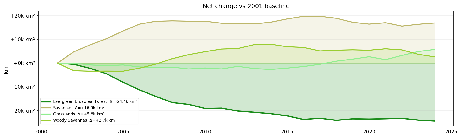
Net land-cover area change relative to the 2001 baseline.

Negative values show loss relative to the first year. Positive values show classes that expanded over the same period.

Step 10. Plot annual forest loss rate

The forest loss rate is calculated from the year-to-year change in forest area.

rate = np.gradient(np.array(forest_km2))

fig, ax = plt.subplots(figsize=(13, 3))

ax.bar(
    years,
    rate,
    color=["#B22222" if value < 0 else "#228B22" for value in rate],
    width=0.7,
    zorder=2,
)

ax.axhline(0, color="#888", lw=0.8)

if len(rate) >= 7:
    ax.plot(
        years,
        savgol_filter(rate, 5, 2),
        color="#222",
        lw=2,
        label="trend",
        zorder=3,
    )

ax.yaxis.set_major_formatter(
    plt.FuncFormatter(lambda value, _: f"{value / 1000:+.1f}k km²/yr")
)

ax.set_title("Annual forest loss rate")
ax.set_ylabel("km²/yr")
ax.legend(fontsize=8)
ax.grid(True, alpha=0.25, axis="y")

fig.tight_layout()
plt.show()

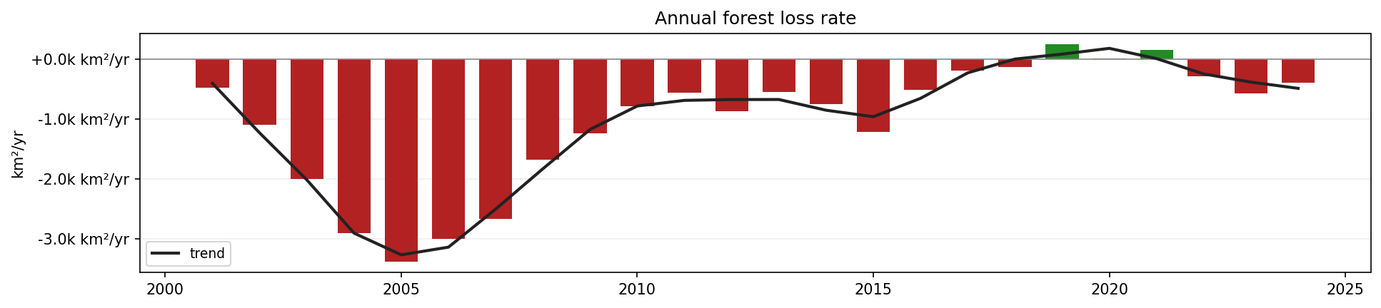
Annual forest loss rate in the selected area of Pará, Brazil.

Red bars indicate annual forest loss. Green bars indicate annual forest gain or classification recovery.

Step 11. Print summary statistics

Finally, print a short numerical summary.

loss = forest_km2[0] - forest_km2[-1]

print(f"Forest {years[0]} : {forest_km2[0]:,.0f} km²")
print(f"Forest {years[-1]} : {forest_km2[-1]:,.0f} km²")
print(f"Loss              : {loss:,.0f} km² ({loss / forest_km2[0] * 100:.1f}%)")
print(f"Peak loss year    : {years[int(np.argmin(rate))]}")

This gives a compact overview of the start value, end value, total forest loss, relative loss, and the year with the strongest single-year decline.

Interpreting the results

The generated outputs provide several views of land-cover change:

• The animated map shows where land-cover changes occurred.

• The stacked area chart shows how the share of each class changed.

• The net area change chart shows the magnitude of forest loss and gains in other classes.

• The annual loss-rate chart shows which years had the strongest forest decline.

• The summary statistics provide a concise numerical interpretation.

The analysis is based on MODIS land-cover classification. It is useful for regional trend analysis, but it does not replace higher-resolution local deforestation mapping.

Limitations

Keep the following limitations in mind:

• MODIS land cover data have a spatial resolution of 500 m.

• Classification errors can occur, especially in mixed pixels and transition zones.

• The workflow uses a rectangular area of interest, not an administrative or ecological boundary.

• The analysis counts classified pixels and does not validate changes against field data.

• S3 credentials are required, and the notebook must be adapted if your S3 endpoint or credential method differs.

Conclusion

In this article, you used a Jupyter Notebook to analyze MODIS land cover change in the Brazilian Amazon. You searched the CREODIAS OData catalogue, downloaded MODIS HDF4 files from S3, processed the LC_Type1 land cover layer, and created charts showing forest-area change and land-cover composition over time.

The same workflow can be adapted to other MODIS tiles, other regions, or other annual land-cover classification products available on Creodias.

What to do next

You can now adapt this workflow to your own analysis. For example, you can:

• change the bounding box to another region,

• use another MODIS tile,

• compare MODIS land cover with Sentinel-2 or Landsat-based classifications,

• replace the rectangular area with a polygon-based area of interest,

• export annual class areas into CSV for reporting,

• combine land-cover change with fire, drought, agriculture, or population data.

You can also continue with other Python and Jupyter Notebook examples in the Cutting Edge section:

• Processing Sentinel-5P data on air pollution using Jupyter Notebook on Creodias

• Analyzing and monitoring floods using Python and Sentinel-2 satellite imagery on Creodias

• Monitoring Urban Sprawl with Sentinel-1 SAR Data Using Pixel Value and Polarization Thresholding on Creodias