MODIS snow cover in Italy analysis using Jupyter Notebook on Creodias

Introduction

This article shows how to analyze MODIS snow cover over the Italian Alps by using a Jupyter Notebook on Creodias. The example uses 8-day maximum snow extent composites from the MODIS MOD10A2 and MYD10A2 products for the period from 2003 to 2022.

The workflow searches the CREODIAS OData catalogue, finds the required MODIS products, resolves their local paths on the virtual machine, and reads the HDF4 files directly from the mounted EODATA filesystem. This avoids downloading large amounts of data before processing and makes the workflow suitable for longer time series.

The area of interest is defined with the local GeoPackage file italian_alps.gpkg. The same polygon is used both for catalogue discovery and for masking pixels outside the Italian Alpine boundary during processing.

Overview

The notebook processes MODIS snow cover data for tile h18v04, which covers the Italian Alps. It reads the Maximum_Snow_Extent layer from each HDF4 file and counts the number of pixels that belong to selected MODIS snow-cover classes.

The main output of the workflow is a set of time series and charts showing how snow and cloud pixels changed over the 2003-2022 period.

The analysis uses the following MODIS pixel classes:

Pixel value	Meaning
200	Snow
25	No snow
50	Cloud
100	Lake ice
37	Open water

What you will do

In this article, you will:

• prepare a Python environment inside a Jupyter Notebook,

• load the Italian Alps area of interest from italian_alps.gpkg,

• search the CREODIAS OData catalogue for MODIS snow products,

• resolve local HDF4 paths on the CREODIAS virtual machine,

• read and process MODIS HDF4 files directly from /eodata,

• count snow, cloud, lake ice, water, and no-snow pixels,

• aggregate the results by year and month,

• create annual, anomaly, heatmap, and decade-comparison charts.

Prerequisites

Before starting, make sure that the following requirements are met.

No. 1 Hosting

You need a Creodias hosting account with access to the Horizon interface:

https://horizon.cloudferro.com/auth/login/?next=/

No. 2 Installing Jupyter Notebook

The code in this article runs in Jupyter Notebook. You can install it on your platform of choice by following the official Jupyter Notebook installation page.

One possible way to run Jupyter Notebook is to install it on a Kubernetes cluster. This is not required for completing this article, but the following article may be useful if you choose that setup:

Installing JupyterHub on Magnum Kubernetes Cluster in Creodias

No. 3 Access to EODATA

The notebook reads MODIS products from EODATA. Make sure that EODATA is available in the environment where you run Jupyter Notebook.

For the MODIS snow article specifically, the notebook reads local file paths from /eodata. Because of that, the first two articles below are the most important: they explain how to mount EODATA as a filesystem on a Linux virtual machine.

The credentials article is useful when the virtual machine does not already have EODATA configured. The Catalogue API manual supports the OData search part of the notebook, where the catalogue is queried before the matching HDF4 files are processed locally.

Depending on how your environment is configured, you may need one of the following articles:

• How to mount EODATA as a filesystem using Goofys in Linux on Creodias

• How to mount eodata using s3fs in Linux on Creodias

• How to get credentials used for accessing EODATA on a cloud VM on Creodias

• EOData Catalogue API Manual on Creodias

No. 4 Required files

This article is accompanied by a ready-to-run Jupyter Notebook and the GeoPackage file used to define the area of interest.

Download both files before running the workflow:

Keep both files in the same working directory. The notebook reads italian_alps.gpkg directly when it loads the Italian Alps area of interest.

The GeoPackage file is used twice in the workflow: first to limit the catalogue search to the selected area, and later to mask MODIS pixels outside the Italian Alps during processing.

Step 1. Install dependencies

The notebook uses Python packages for catalogue access, geospatial processing, HDF4 reading, plotting, and statistics.

Run the following cell at the beginning of the notebook:

import importlib, subprocess, sys

pkgs = ["rasterio", "pyhdf", "scipy", "geopandas", "shapely"]
missing = [p for p in pkgs if importlib.util.find_spec(p) is None]

if missing:
    subprocess.check_call([sys.executable, "-m", "pip", "install", "-q"] + missing)

The packages are used as follows:

Package	Purpose
pyhdf	Reads HDF4 files produced by MODIS.
geopandas and shapely	Load the area of interest from the GeoPackage file and prepare the polygon.
rasterio	Rasterizes the area-of-interest polygon into a pixel mask.
scipy	Calculates the linear trend and moving averages.
matplotlib	Creates the charts in the notebook.

Step 2. Import libraries and define global settings

After the packages are available, import the required Python modules and define the global parameters used by the workflow.

import os
import gc
import time
import requests
import numpy as np
import matplotlib.pyplot as plt
import matplotlib.patches as mpatches
import geopandas as gpd

from shapely.geometry import mapping
from rasterio.transform import from_bounds
from rasterio.features import geometry_mask
from pyhdf.SD import SD, SDC
from datetime import datetime
from collections import defaultdict
from concurrent.futures import ThreadPoolExecutor, as_completed
from IPython.display import clear_output
from scipy import stats
from pathlib import Path

MAX_WORKERS = min(8, os.cpu_count() or 4)
GC_EVERY = 50
LAYER = "Maximum_Snow_Extent"

print(f"ready | workers={MAX_WORKERS} | layer={LAYER}")

The most important setting is LAYER. It defines the scientific dataset that will be read from each MODIS HDF4 file.

Step 3. Load the Italian Alps area of interest

The area of interest is stored in italian_alps.gpkg. The notebook loads this file, reprojects it to WGS84 if needed, dissolves all features into one geometry, and extracts the bounding box for catalogue search.

BASE_DIR = Path.cwd()
GPKG_PATH = BASE_DIR / "italian_alps.gpkg"

if not GPKG_PATH.exists():
    print(f"Warning: {GPKG_PATH} not found!")

aoi_gdf = gpd.read_file(GPKG_PATH)

if aoi_gdf.crs is None or aoi_gdf.crs.to_epsg() != 4326:
    aoi_gdf = aoi_gdf.to_crs(epsg=4326)

aoi_union = aoi_gdf.geometry.unary_union
aoi_geojson = mapping(aoi_union)

AOI_MINX, AOI_MINY, AOI_MAXX, AOI_MAXY = aoi_union.bounds

print(f"Loaded  : {GPKG_PATH}")
print(f"CRS     : {aoi_gdf.crs}")
print(f"Features: {len(aoi_gdf)}")
print(
    f"BBox    : lon [{AOI_MINX:.3f}, {AOI_MAXX:.3f}] "
    f"lat [{AOI_MINY:.3f}, {AOI_MAXY:.3f}]"
)

Display the polygon to verify that the correct area has been loaded:

fig, ax = plt.subplots(figsize=(8, 4))
aoi_gdf.plot(ax=ax, facecolor="#cce5ff", edgecolor="#185FA5", linewidth=0.8)

ax.set_title("AOI - Italian Alps from GeoPackage", fontsize=10)
ax.set_xlabel("Longitude")
ax.set_ylabel("Latitude")

plt.tight_layout()
plt.show()

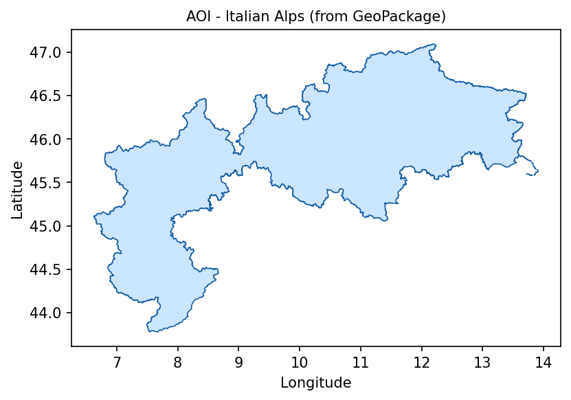
Italian Alps area of interest loaded from italian_alps.gpkg.

At this point, the notebook has the polygon that will be used both for catalogue search and for pixel masking. This is important because the MODIS tile is larger than the Italian Alps. Without the mask, lowland and coastal areas outside the Alpine region would influence the statistics.

Step 4. Search the OData catalogue

The notebook searches the CREODIAS OData catalogue for MODIS snow products:

https://datahub.creodias.eu/odata/v1/Products

The workflow searches two products:

• MOD10A2 from Terra,

• MYD10A2 from Aqua.

Both are 8-day maximum snow extent products. The query is limited to MODIS tile h18v04 and to the 2003-2022 eriod.

First, define the catalogue endpoint and the area-of-interest polygon in WKT format:

ODATA_BASE = "https://datahub.creodias.eu/odata/v1/Products"

aoi_wkt = (
    f"POLYGON(("
    f"{AOI_MINX} {AOI_MINY},"
    f"{AOI_MAXX} {AOI_MINY},"
    f"{AOI_MAXX} {AOI_MAXY},"
    f"{AOI_MINX} {AOI_MAXY},"
    f"{AOI_MINX} {AOI_MINY}"
    f"))"
)

Create a helper function that builds the OData filter:

def build_filter(collection: str, product_name: str) -> str:
    return (
        f"Collection/Name eq '{collection}'"
        f" and contains(Name,'{product_name}')"
        " and contains(Name,'h18v04')"
        " and ContentDate/Start gt 2003-01-01T00:00:00.000Z"
        " and ContentDate/Start lt 2023-01-01T00:00:00.000Z"
        f" and OData.CSC.Intersects(area=geography'SRID=4326;{aoi_wkt}')"
    )

The next helper function retrieves all result pages. Results are requested in batches of 100 products and sorted by acquisition date.

def fetch_all_pages(odata_filter: str) -> list:
    products = []
    skip, PAGE = 0, 100

    while True:
        params = {
            "$filter": odata_filter,
            "$orderby": "ContentDate/Start asc",
            "$top": PAGE,
            "$skip": skip,
            "$expand": "Locations",
        }

        resp = requests.get(ODATA_BASE, params=params, timeout=60)
        resp.raise_for_status()

        page = resp.json().get("value", [])
        products.extend(page)

        if len(page) < PAGE:
            break

        skip += PAGE

    return products

Run the search for both Terra and Aqua products:

print("Querying OData catalogue for MOD10A2 Terra ...")
mod_products = fetch_all_pages(build_filter("TERRA", "MOD10A2"))
print(f"  -> {len(mod_products)} items")

print("Querying OData catalogue for MYD10A2 Aqua ...")
myd_products = fetch_all_pages(build_filter("AQUA", "MYD10A2"))
print(f"  -> {len(myd_products)} items")

all_products = sorted(
    mod_products + myd_products,
    key=lambda p: p["ContentDate"]["Start"]
)

print(f"\nTotal items found : {len(all_products)}")

if all_products:
    print(
        f"Date range        : "
        f"{all_products[0]['ContentDate']['Start'][:10]} -> "
        f"{all_products[-1]['ContentDate']['Start'][:10]}"
    )

The resulting all_products list contains the catalogue metadata needed for processing. Because the query uses $expand=Locations, each product also contains the location information used to resolve the local HDF4 file path.

Step 5. Read and process the HDF4 files

The MODIS files are read directly from the EODATA filesystem mounted on the virtual machine. There is no separate download step.

For each product, the notebook:

1. resolves the local filesystem path from the product metadata,

2. opens the HDF4 file,

3. reads only the window that overlaps the area of interest,

4. applies the Italian Alps polygon mask,

5. counts pixels by MODIS snow-cover class,

6. returns one statistics record per MODIS composite.

Define a helper function that finds the local HDF4 file for a product:

def local_path_from_product(product: dict):
    """Return path to the .hdf file inside the scene directory, or None."""
    for loc in product.get("Locations", []):
        if loc.get("FormatType") == "Extracted" and loc.get("S3Path"):
            scene_dir = loc["S3Path"]

            try:
                for fname in os.listdir(scene_dir):
                    if fname.lower().endswith(".hdf"):
                        return os.path.join(scene_dir, fname)
            except OSError:
                return None

    return None

Define a helper function that extracts the tile bounds from the product footprint:

def _tile_bbox(product: dict) -> tuple[float, float, float, float]:
    """Parse tile bounds from product footprint WKT; fall back to h18v04 defaults."""
    tile_minx, tile_maxx = 0.0, 20.0
    tile_miny, tile_maxy = 40.0, 60.0

    if product.get("Footprint"):
        try:
            wkt = product["Footprint"]

            if ";" in wkt:
                wkt = wkt.split(";", 1)[1].strip().rstrip("'")

            coords_str = wkt.split("((")[1].split("))")[0]
            coords = [
                tuple(map(float, p.strip().split()))
                for p in coords_str.split(",")
            ]

            lons = [c[0] for c in coords]
            lats = [c[1] for c in coords]

            tile_minx, tile_maxx = min(lons), max(lons)
            tile_miny, tile_maxy = min(lats), max(lats)

        except Exception:
            pass

    return tile_minx, tile_maxx, tile_miny, tile_maxy

Before processing all products, compute the shape of the array window that overlaps the area of interest:

def _window_shape() -> tuple[int, int]:
    """Scan products to determine the row and column size of the AOI clip window."""
    for p in all_products:
        if local_path_from_product(p) is None:
            continue

        tile_minx, tile_maxx, tile_miny, tile_maxy = _tile_bbox(p)

        h = w = 1200

        col0 = max(0, min(w, int((AOI_MINX - tile_minx) / (tile_maxx - tile_minx) * w)))
        col1 = max(0, min(w, int((AOI_MAXX - tile_minx) / (tile_maxx - tile_minx) * w)))
        row0 = max(0, min(h, int((tile_maxy - AOI_MAXY) / (tile_maxy - tile_miny) * h)))
        row1 = max(0, min(h, int((tile_maxy - AOI_MINY) / (tile_maxy - tile_miny) * h)))

        if col1 > col0 and row1 > row0:
            return row1 - row0, col1 - col0

    raise RuntimeError("Could not determine window shape from any product.")

Build the AOI mask once. This avoids rasterizing the polygon again for every MODIS file.

nrows, ncols = _window_shape()

_transform = from_bounds(
    AOI_MINX,
    AOI_MINY,
    AOI_MAXX,
    AOI_MAXY,
    ncols,
    nrows
)

AOI_MASK_OUTSIDE = geometry_mask(
    [aoi_geojson],
    transform=_transform,
    invert=False,
    out_shape=(nrows, ncols)
)

print(
    f"AOI mask computed: {nrows}x{ncols} px "
    f"({AOI_MASK_OUTSIDE.sum()} px outside AOI)"
)

Now define the processing function for one product:

def process_product(product: dict):
    """Read one HDF scene, clip it to the AOI, and count pixels by class."""
    hdf = sds = None

    try:
        local_path = local_path_from_product(product)

        if local_path is None:
            return None

        tile_minx, tile_maxx, tile_miny, tile_maxy = _tile_bbox(product)

        h = w = 1200

        col0 = max(0, min(w, int((AOI_MINX - tile_minx) / (tile_maxx - tile_minx) * w)))
        col1 = max(0, min(w, int((AOI_MAXX - tile_minx) / (tile_maxx - tile_minx) * w)))
        row0 = max(0, min(h, int((tile_maxy - AOI_MAXY) / (tile_maxy - tile_miny) * h)))
        row1 = max(0, min(h, int((tile_maxy - AOI_MINY) / (tile_maxy - tile_miny) * h)))

        if col1 <= col0 or row1 <= row0:
            return None

        hdf = SD(local_path, SDC.READ)
        sds = hdf.select(LAYER)
        arr = sds[row0:row1, col0:col1]

        if arr.shape != AOI_MASK_OUTSIDE.shape:
            t = from_bounds(
                AOI_MINX,
                AOI_MINY,
                AOI_MAXX,
                AOI_MAXY,
                arr.shape[1],
                arr.shape[0]
            )

            mask = geometry_mask(
                [aoi_geojson],
                transform=t,
                invert=False,
                out_shape=arr.shape
            )
        else:
            mask = AOI_MASK_OUTSIDE

        arr = np.where(mask, 0, arr)

        snow_px = int(np.sum(arr == 200))
        no_snow_px = int(np.sum(arr == 25))
        cloud_px = int(np.sum(arr == 50))
        lake_ice_px = int(np.sum(arr == 100))
        lake_px = int(np.sum(arr == 37))

        if snow_px + no_snow_px + cloud_px + lake_ice_px + lake_px == 0:
            return None

        dt = datetime.fromisoformat(
            product["ContentDate"]["Start"].replace("Z", "+00:00")
        )

        platform = "terra" if "MOD10A2" in product["Name"] else "aqua"

        return {
            "dt": dt,
            "year": dt.year,
            "month": dt.month,
            "doy": dt.timetuple().tm_yday,
            "platform": platform,
            "snow_px": snow_px,
            "no_snow_px": no_snow_px,
            "cloud_px": cloud_px,
            "lake_ice_px": lake_ice_px,
            "lake_px": lake_px,
        }

    except Exception:
        return None

    finally:
        try:
            if sds:
                sds.endaccess()
        except Exception:
            pass

        try:
            if hdf:
                hdf.end()
        except Exception:
            pass

Process all products in parallel:

results = []
t_start = datetime.now()
processed = 0
last_print_t = time.time()

PRINT_EVERY = 25
PRINT_EVERY_S = 5
total = len(all_products)

with ThreadPoolExecutor(max_workers=MAX_WORKERS) as executor:
    futures = {executor.submit(process_product, p): p for p in all_products}

    for future in as_completed(futures):
        processed += 1
        result = future.result()

        if result is not None:
            results.append(result)

        now = time.time()

        if (
            processed % PRINT_EVERY == 0
            or (now - last_print_t) >= PRINT_EVERY_S
            or processed == total
        ):
            skipped = processed - len(results)
            elapsed = (datetime.now() - t_start).total_seconds()
            rate = processed / elapsed if elapsed > 0 else 0.0
            eta = (total - processed) / rate if rate > 0 else 0.0
            pct = processed / total
            bar = "█" * int(pct * 30) + "░" * (30 - int(pct * 30))

            clear_output(wait=True)

            print(
                f"[{bar}] {processed}/{total} ({pct * 100:.1f}%)\n"
                f"  ok={len(results)}  skip={skipped}\n"
                f"  elapsed={elapsed:.1f}s  rate={rate:.1f} file/s  ETA={eta:.0f}s",
                flush=True
            )

            last_print_t = now

        if processed % GC_EVERY == 0:
            gc.collect()

gc.collect()

results = sorted(results, key=lambda x: x["dt"])
t_total = (datetime.now() - t_start).total_seconds()

print(f"\nDone - {len(results)} results, {len(all_products) - len(results)} skipped")
print(
    f"  Total time : {t_total:.1f}s "
    f"({t_total / max(len(all_products), 1) * 1000:.0f} ms/file avg)"
)

The results list now contains one processed record per valid MODIS composite.

Step 6. Build aggregate time series

The next step converts the per-product pixel counts into annual and monthly summary datasets.

The notebook calculates:

• the number of 8-day composites with snow pixels above the selected threshold,

• the estimated snow-season length in days,

• the anomaly from the 2003-2022 mean,

• monthly snow-pixel totals for heatmap and decade comparison charts,

• a linear trend over the full period.

SNOW_THRESHOLD = 50

yearly_snow_composites = defaultdict(int)
yearly_snow_total = defaultdict(int)
yearly_cloud_total = defaultdict(int)
yearly_composite_count = defaultdict(int)

monthly_snow: dict[int, dict[int, list]] = {}

for r in results:
    y, m = r["year"], r["month"]

    yearly_composite_count[y] += 1
    yearly_cloud_total[y] += r["cloud_px"]
    yearly_snow_total[y] += r["snow_px"]

    if r["snow_px"] > SNOW_THRESHOLD:
        yearly_snow_composites[y] += 1

    monthly_snow.setdefault(y, {}).setdefault(m, []).append(r["snow_px"])

years = sorted(yearly_snow_composites.keys())
season_days = {y: yearly_snow_composites[y] * 8 for y in years}
season_arr = np.array([season_days[y] for y in years])

baseline_mean = np.mean([season_days[y] for y in years])

anomaly_pct = {
    y: (season_days[y] - baseline_mean) / baseline_mean * 100
    for y in years
}

x_idx = np.arange(len(years))
slope, intercept, r_val, *_ = stats.linregress(x_idx, season_arr)
trend_line = slope * x_idx + intercept

def moving_avg(arr, w=5):
    return [
        np.mean(arr[max(0, i - w // 2): i + w // 2 + 1])
        for i in range(len(arr))
    ]

mov_avg = moving_avg(season_arr)

print(f"Years in analysis : {years[0]}-{years[-1]}")
print(f"Baseline mean     : {baseline_mean:.0f} snow-days/yr (2003-2022)")
print(f"Linear trend      : {slope * 10:.1f} days per decade (R2={r_val ** 2:.3f})")

The result is not a physical snow-depth measurement. It is a time series based on classified MODIS pixels inside the Italian Alps polygon. It is useful for observing broad seasonal and multi-year patterns.

Step 7. Plot annual snow and cloud pixels

The first chart compares annual snow-pixel and cloud-pixel totals. Cloud coverage is shown because it can affect the interpretation of snow extent.

BLUE_DARK = "#185FA5"
BLUE_MID = "#378ADD"
BLUE_LIGHT = "#85B7EB"
BLUE_PALE = "#B5D4F4"
BLUE_DEEP = "#0C447C"
RED = "#E24B4A"

x, bar_w = np.arange(len(years)), 0.4

fig, ax = plt.subplots(figsize=(15, 5))

ax.bar(
    x - bar_w / 2,
    [yearly_snow_total[y] for y in years],
    bar_w,
    label="Snow pixels (200)",
    color=BLUE_DARK
)

ax.bar(
    x + bar_w / 2,
    [yearly_cloud_total[y] for y in years],
    bar_w,
    label="Cloud pixels (50)",
    color=BLUE_PALE
)

ax.set_xticks(x)
ax.set_xticklabels(years, rotation=45, ha="right")
ax.set_xlabel("Year")
ax.set_ylabel("Total pixel count")
ax.set_title("Annual snow and cloud pixels - Italian Alps (2003-2022)")
ax.legend(fontsize=9)
ax.grid(True, alpha=0.25, axis="y")

fig.tight_layout()
plt.show()

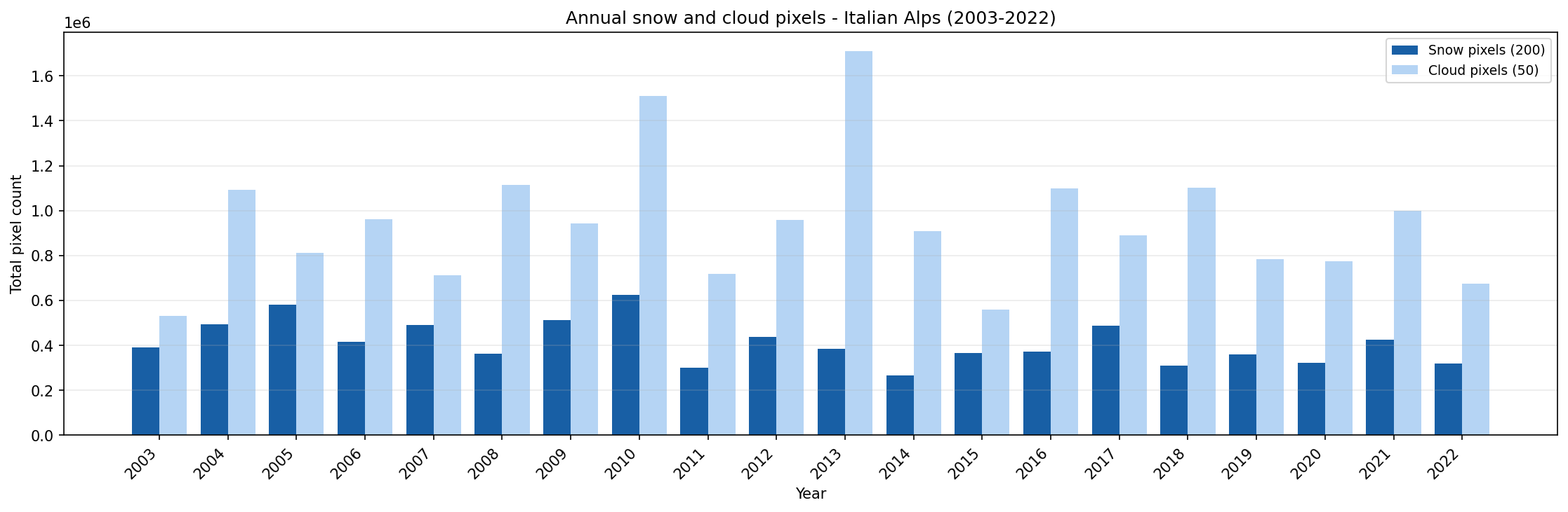
Annual snow and cloud pixel totals for the Italian Alps from 2003 to 2022.

Use this chart to compare years with high and low snow-pixel counts. Years with high cloud-pixel totals should be interpreted more carefully, because cloud cover can hide the actual snow surface.

Step 8. Plot annual snow anomaly

The second chart shows the percentage difference between each year and the 2003-2022 mean snow-season length.

anom_vals = [anomaly_pct[y] for y in years]
bar_colors = [BLUE_DARK if v >= 0 else RED for v in anom_vals]
x = np.arange(len(years))

fig, ax = plt.subplots(figsize=(15, 5))

bars = ax.bar(
    x,
    anom_vals,
    color=bar_colors,
    width=0.7,
    zorder=2
)

ax.axhline(0, color="#888", lw=0.8)
ax.set_xticks(x)
ax.set_xticklabels(years, rotation=45, ha="right")
ax.yaxis.set_major_formatter(plt.FuncFormatter(lambda v, _: f"{v:+.0f}%"))

for bar, v in zip(bars, anom_vals):
    offset = 0.4 if v >= 0 else -0.4
    va = "bottom" if v >= 0 else "top"

    ax.text(
        bar.get_x() + bar.get_width() / 2,
        v + offset,
        f"{v:+.1f}%",
        ha="center",
        va=va,
        fontsize=6.5,
        color="#333"
    )

ax.set_xlabel("Year")
ax.set_ylabel("Anomaly vs 2003-2022 mean")
ax.set_title("Annual snow anomaly - Italian Alps (2003-2022)")
ax.grid(True, alpha=0.2, axis="y")

p1 = mpatches.Patch(color=BLUE_DARK, label="above mean")
p2 = mpatches.Patch(color=RED, label="below mean")

ax.legend(handles=[p1, p2], fontsize=9)

fig.tight_layout()
plt.show()

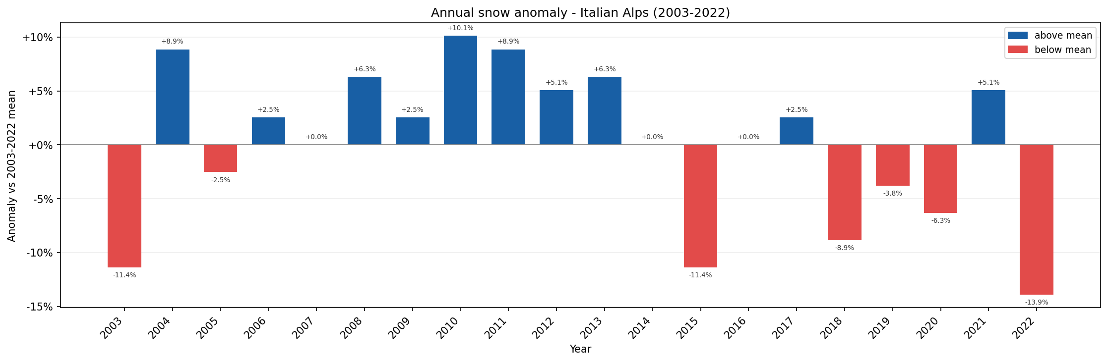
Annual snow anomaly for the Italian Alps compared with the 2003-2022 mean.

In this chart:

• blue bars show years with above-average snow-season length,

• red bars show years with below-average snow-season length.

Step 9. Plot the year-month heatmap

The heatmap compresses the full time series into one view. Each row represents a year and each column represents a month.

all_years = sorted(monthly_snow.keys())

month_names = [
    "Jan", "Feb", "Mar", "Apr", "May", "Jun",
    "Jul", "Aug", "Sep", "Oct", "Nov", "Dec"
]

matrix = np.array(
    [
        [sum(monthly_snow[y].get(m, [0])) for m in range(1, 13)]
        for y in all_years
    ],
    dtype=float
)

fig, ax = plt.subplots(figsize=(13, 7))

im = ax.imshow(
    matrix,
    aspect="auto",
    cmap="Blues",
    interpolation="nearest"
)

plt.colorbar(im, ax=ax, label="Total snow pixels")

ax.set_yticks(range(len(all_years)))
ax.set_yticklabels(all_years, fontsize=9)
ax.set_xticks(range(12))
ax.set_xticklabels(month_names)
ax.set_title("Snow cover heatmap - Italian Alps: year x month (2003-2022)")

fig.tight_layout()
plt.show()

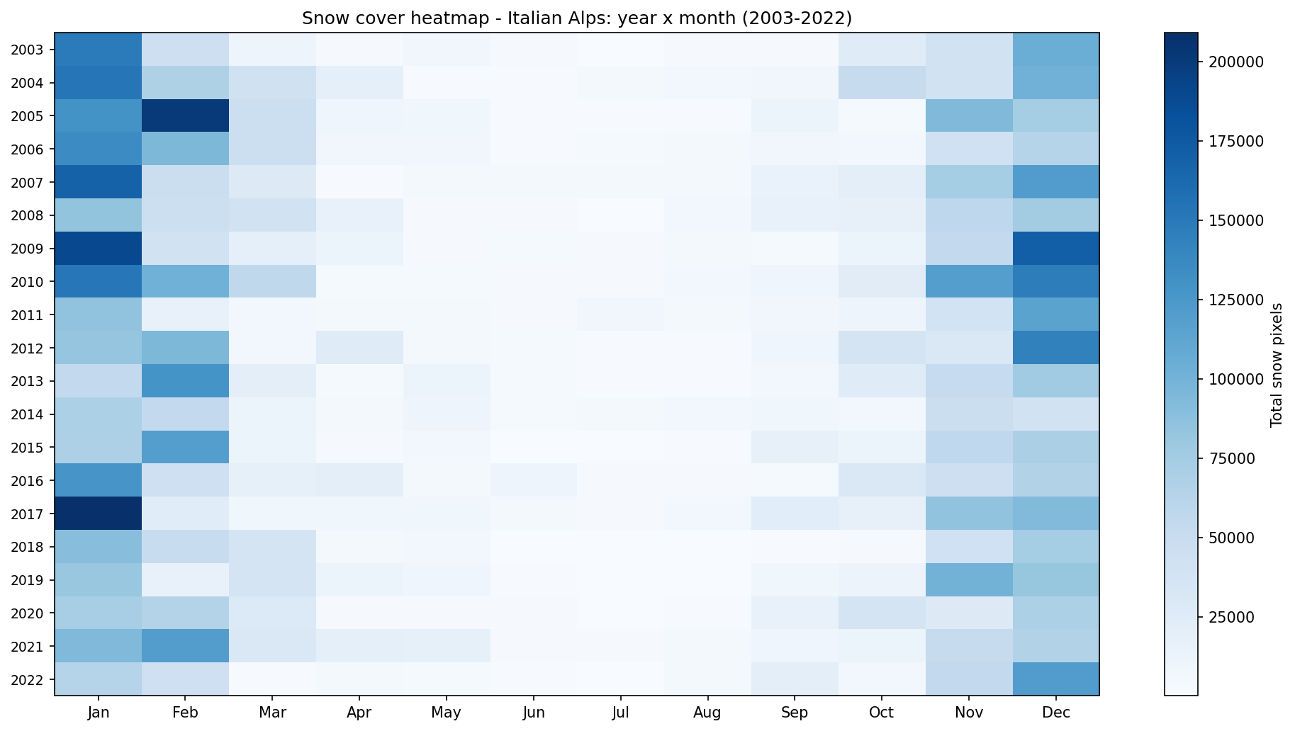
Monthly snow cover heatmap for the Italian Alps from 2003 to 2022.

Bright cells indicate higher snow-pixel totals. In a typical Alpine pattern, snow is concentrated in the cold season, while summer months should show little or no snow.

Step 10. Compare monthly snow profiles by decade

The final chart compares the mean monthly snow-pixel count for two decades: 2003-2012 and 2013-2022.

decades = {
    "2003-2012": [y for y in years if 2003 <= y <= 2012],
    "2013-2022": [y for y in years if 2013 <= y <= 2022],
}

decade_colors = {
    "2003-2012": BLUE_DEEP,
    "2013-2022": BLUE_LIGHT,
}

x, bar_w = np.arange(12), 0.35

fig, ax = plt.subplots(figsize=(13, 5))

for i, (label, dec_years) in enumerate(decades.items()):
    means = []

    for m in range(1, 13):
        vals = [
            v
            for y in dec_years
            for v in monthly_snow[y].get(m, [])
        ]

        means.append(np.mean(vals) if vals else 0)

    ax.bar(
        x + (i - 0.5) * bar_w,
        means,
        bar_w,
        color=decade_colors[label],
        label=label
    )

ax.set_xticks(x)
ax.set_xticklabels(month_names)
ax.set_ylabel("Mean snow pixels per 8-day composite")
ax.set_title("Monthly snow profile by decade - Italian Alps (2003-2022)")
ax.legend(fontsize=9)
ax.grid(True, alpha=0.2, axis="y")

fig.tight_layout()
plt.show()

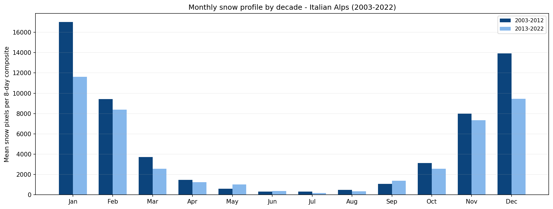
Monthly snow profile comparison for 2003-2012 and 2013-2022.

This chart helps identify whether snow cover is changing between the two periods. For example, a lower spring value in the second decade may suggest earlier melting, while a lower winter value may indicate a generally weaker snow season.

Interpreting the results

The generated charts provide a compact overview of snow-cover behavior in the Italian Alps over a 20-year period.

Use them as follows:

• The annual snow and cloud pixel chart helps compare snow and cloud totals across years.

• The annual anomaly chart highlights years that were above or below the long-term mean.

• The heatmap shows the seasonal distribution of snow pixels across the full record.

• The decade comparison chart shows whether the monthly snow profile changed between 2003-2012 and 2013-2022.

The analysis is based on classified MODIS pixels. It does not replace local snow-depth measurements or meteorological records, but it gives a useful satellite-based view of regional snow-cover patterns.

Limitations

Keep the following limitations in mind:

• MODIS snow products have a spatial resolution of 500 m, which is suitable for regional analysis but not for very local terrain features.

• Cloud cover can hide snow and influence annual or monthly statistics.

• The workflow counts classified pixels; it does not estimate snow depth or snow water equivalent.

• The analysis uses one MODIS tile and one area-of-interest polygon. Changing the region may require changing the tile filter and the GeoPackage file.

• The notebook reads files directly from /eodata, so it must be adapted if you want to run it outside the Creodias environment.

Conclusion

In this article, you used a Jupyter Notebook to analyze 20 years of MODIS snow cover over the Italian Alps. You searched the CREODIAS OData catalogue, resolved the matching HDF4 files on the EODATA filesystem, processed the Maximum_Snow_Extent layer, and created charts showing annual, monthly, and decadal snow-cover patterns.

The same structure can be reused for other MODIS products, other areas of interest, or other Earth observation datasets available on Creodias.

What to do next

You can now adapt this workflow to your own analysis. For example, you can:

• replace italian_alps.gpkg with another area-of-interest file,

• change the MODIS tile filter if your region is located in another tile,

• modify the date range,

• compare Terra and Aqua results separately,

• combine MODIS snow cover with elevation data or other environmental datasets,

• export the aggregated results for reporting or dashboard use.

You can also continue with other Python and Jupyter Notebook examples in the Cutting Edge section:

• Processing Sentinel-5P data on air pollution using Jupyter Notebook on Creodias

• Analyzing and monitoring floods using Python and Sentinel-2 satellite imagery on Creodias

• Monitoring Urban Sprawl with Sentinel-1 SAR Data Using Pixel Value and Polarization Thresholding on Creodias